Download
1 / 48
480 likes | 532 Views
Explore simple linear regression using porosity and strength data of pencil lead. Learn how to estimate and test the relationship.

E N D
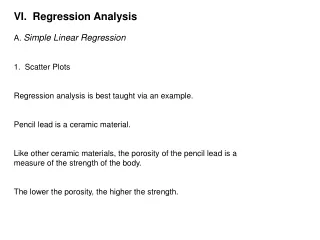
VI. Regression Analysis A. Simple Linear Regression 1. Scatter Plots Regression analysis is best taught via an example. Pencil lead is a ceramic material. Like other ceramic materials, the porosity of the pencil lead is a measure of the strength of the body. The lower the porosity, the higher the strength.
The following data are the porosities and strengths for a popular # 2 pencil lead.
First, consider a scatter plot of these data. As expected, the plot suggests that as the porosity gets smaller, the strength gets larger (a negative relationship). We also see that the relationship is not perfect (the data do not form a perfect straight line). The data exhibit some “noise” or variability around the possible linear relationship.
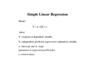
2. The Simple Linear Regression Model • Suppose we believe that as at least a first approximation, there is a strictly linear relationship between strength and porosity. • What is the appropriate model? • where • yi is the response, in this case, the strength of the ith pencil lead, • xi is the predictor or regressor, in this case, the porosity of the ith pencil lead, • is the y-intercept, • is the slope (in our case, we expect to be negative), and • is a random error.
We usually assume that the random errors are independent and that they all have an expected value of 0 and variance σ2. • With these assumptions, • which is a straight line. • The statistical model represents the approximate relationship between yi, the response of interest, and the xi which is the regressor. • By knowing , we know the relationship between y and x. • If , then there is a negative relationship between yi and xi. • If , then there is a positive relationship. • If , then there is no relationship!
Problem: Do we ever know or ? How should we choose our estimates for and ? Since is a straight line, we should choose our estimates to produce the “best” line through the data. Note: There are an infinite number of possible lines. How shall we define the “best” line?
3. Least Squares Estimation • Consider an estimated relationship between y and x given by • Note: • is an estimate or prediction of yi. • b0 is an estimate of the y-intercept. • b1 is an estimate of the slope.
One possible line through our scatter plot is the following.
Consider the difference between each actual observation yi and its predicted value, . We usually call this difference the ith residual, ei; thus, For a good estimated line, all of the residuals should be “small”. Thus, one possible measure of how good our estimated line is Problem: Note, for some data points ei < 0, for others, ei > 0. A poor fit where ei is much less than 0 can be compensated by another very poor fit when ei is much larger than 0. Thus, is not a particularly good measure.
A better measure? which we call the sum of squares for the residuals (SSres). Our best estimated line, then, is the one which minimizes SSres. Therefore we wish to choose b0 and b1 such that SSres is minimized. What values of b0 and b1 accomplish this? We need to return to basic calculus.
where and
Therefore, our prediction equation is The following is a plot of this prediction equation through the actual data.
4. Hypothesis Tests for Usually, the most important question to be addressed by regression analysis is whether the slope is 0. Our approach for answering this question: a hypothesis test. 1. State the hypotheses. Note: Most statistical software packages assume . 2. State the test statistic. To obtain the test statistic, we need to understand the distribution of b1.
If the random errors, the ε’s, follow a normal distribution with mean 0 and variance σ2, then also follows a normal distribution with a mean of β1 and a variance of Note: b1 is an unbiased estimator of β1. Problem: Do we know σ2? Of course, not. Therefore to develop an appropriate test statistic, we first need to develop an appropriate estimate for σ2.
We shall use Why use the denominator n-2? The denominator for our variance estimators is always the appropriate degrees of freedom (df). The appropriate degrees of freedom is always given by df = (number of observations used) - (number of parameter estimates required)
Look at SSres. Note: We must estimate both β0 and β1 to calculate SSres; thus, df = n - 2 . To compute MSres, we need a better way to find SSres. The definitional formula for SSres is
The computational formula is given by SSres = SStotal - b1 SSxy where Thus, an appropriate estimate of the variance of b1 is given by An appropriate test statistic is This t statistic has n-2 degrees of freedom.
We may also express this test statistic as where is the estimated standard error for b1. Most software packages report b1 and , which allows the analyst to compute the t statistic from the output. 3. State the rejection region. Rejection Regions are just as before. Thus, if , then we reject H0 if . If , we reject H0 if . If , we reject H0 if . Steps 4 and 5 are the same as before.
Return to our example: Perform the appropriate test for using a .05 significance level. 1. State the hypotheses. 2. State the test statistic. In this case, the test statistic is 3. State the critical region. In this case, we reject H0 if
Since n = 10, we reject H0 if 4. Conduct experiment and calculate the test statistic.
5. Reach conclusions. t is not < -1.860 Therefore we must fail to reject H0. Thus, we have insufficient evidence to establish that there is negative linear relationship between porosity and strength. Since we failed to reject the claim that there is no relationship, we are not required to calculate a confidence interval for . In general, however, we can construct a (1 - ) •100% confidence interval for by
For our specific case, a 95% confidence interval for is which clearly includes 0.
5. The Coefficient of Determination, R2 • We can partition the total variability in the data, SStotal into two components: • SSreg, the sum of squares due to the regression model, and • SSres, which is the sum of squares due to the residuals. • We define by SSreg • SSreg represents the variability in the data explained by our model. • SSres represents the variability unexplained and presumed due to error.
Note: If our model fits the data well, then • SSreg should be “large”, and • SSres should be near 0. • On the other hand, if the model does not fit the data well, then • SSreg should be near 0, and • SSres should be large. • One reasonable measure of the overall performance of our model is the coefficient of determination, R2, given by • It can be shown that 0 ≤ R2 ≤ 1.
Note: If the fit is good, SSres is near 0 and R2 is near 1. If the fit is poor, SSres is large and R2 is near 0. A problem with R2 : What defines a good value? The answer depends upon the application area. Typically, in many engineering problems, R2 > .9 However, there are some very “noisy” systems where a good R2 is .20.
We generally use the computational formula to compute SSreg, which is For our example: SStotal = 0.159, b1 = -0.265, and SSxx = 0.585. Thus, and which is rather poor and confirms our hypothesis test.
6. The Overall F-Test This procedure focuses purely on whether some relationship, either positive or negative, exists between the response and the regressor. Consequently, it is inherently a two-sided procedure. In general, this test evaluates the overall adequacy of the model. For simple linear regression, this test reduces to a two-sided test for the slope, in which case, our hypotheses are In multiple regression, this test simultaneously evaluates all of the slopes.
Our test statistic is based on MSreg which is defined by where dfreg = the number of regressors In the case of simple linear regression, dfreg = 1. Our test statistic is The degrees of freedom for the test statistic are 1 for the numerator and n-2 for the denominator. One way to view this F statistics is as a signal-to-noise ratio. MSreg is a standardized measure of what the model explains (a signal). MSres is a standardized measure of the error (a measure of noise).
Since we have only one possible alternative hypothesis, we always reject H0 if . In our case, we reject the null hypothesis if For our example SSreg = 0.041 and dfreg = 1. Thus,
Since MSres = 0.01474, our test statistic is Apart from rounding errors, this value for the F statistic is the square of the value for the t statistic we used to test the slope originally. We typically use the following analysis of variance (ANOVA) table to summarize the calculations for this test. Degrees of Sum of Mean Source Freedom Squares Squares F Regression dfregSSregMSregF Residual dfresSSresMSres Total n-1 SStotal
For our specific situation, the ANOVA table is the following. Degrees of Sum of Mean Source Freedom Squares Squares F Regression 1 0.041 0.041 2.782 Residual 8 0.118 0.01474 Total 9 0.159 Source refers to our partition of the total variability into two components: one for the regression model, and the other for the residual or error. For simple linear regression, the degrees of freedom for the model are number of parameters - 1 = 2 - 1 = 1 .
The degrees of freedom for the residuals for this particular situation are number of observations - number of parameters = n - 2 = 8 . We obtain the mean squares by dividing the appropriate sum of squares by the corresponding degrees of freedom. We calculate the F statistic by dividing the mean square for regression by the mean square for the residuals. Since 2.782 is not > 5.32, we cannot reject the null hypothesis that porosity and strength are not related.
7. Reading a Computer Generated Analysis Repeat the analysis of the porosity and strength data using the software package of your choice. Highlight all of the tests we did by hand. If your software allows you to calculate confidence and prediction bands, then do so.
C. Multiple Linear Regression Choose either one of the exercises from the book that you do not assign for homework or a data set of your own to illustrate multiple linear regression. Do all of the analysis within the software package of your choice. Continually emphasize that multiple linear regression is a straight forward extension of simple linear regression. We spent a lot of time in simple linear regression laying the necessary foundations for multiple linear regression. Once students understand reading the computer output for simple linear regression, they can pick up very quickly how to read the output for multiple linear regression.
The following questions should guide your discussion of the example: • 1. What is our model and how should we estimate it? • 2. What is the overall adequacy of our model? • 3. Which specific regressors seem important? • Once we begin residual analysis, we shall add the following questions: • Is the model reasonable correct? • How well do our data meet the assumptions required for our analysis?
Highlight the following: • 1. The model. • where • yi is the ith response, • xij is the ith value for the jth regressor, • k is the number of regressors, • β0 is the y-intercept, • βj is coefficient associated with the jth regressor, and • εi is a random error with mean 0 and constant variance σ2.
Again, emphasize the extension from simple linear regression. Be sure to emphasize that we can no longer call the βj's slopes. The βj's represent the expected change in y given a one unit change in xjif we hold all of the other regressors constant.
2. We estimate the model using least squares. • The estimated model is • where • is the predicted response, • b0 is the estimated y-intercept, and • bj is the estimated coefficient for the jth regressor. • In multiple regression, we once again find the b's which minimize • In this course, we always let computer software packages perform the estimation.
3. We determine the overall adequacy of the model in two ways. First, the multiple coefficient of determination, R2, given by where which is the same way that we defined the coefficient of determination for simple linear regression. Second, the overall F test, which test the hypotheses
The test statistic is based on MSreg and MSres, which are defined just as they were for simple linear regression; thus, where dfreg is the number of regressors, and where dfres is the number of observations (n) minus the number of parameters estimated (k+1); thus, dfres = n-k-1 . The test statistic is and has k numerator degrees of freedom and n-k-1 denominator degrees of freedom.
4. We determine whether a specific regressor makes a significant contribution through t-tests of the form The test statistics have the form It is important to note that these tests actually are tests on the contribution of the specific regressor given that all of the other regressors are in the model. Thus, these tests do not determine whether the specific regressor is important in isolation from the effects of the other regressors. This point emphasizes why we cannot call the β's slopes! Again, we let computer software packages perform this task.
D. Residual Analysis Continue the multiple regression analysis by checking the model assumptions using proper residual analysis. Again, do all of the calculations and plotting using the software package of choice. If you have the option, use the studentized residuals rather than the raw or standardized residuals.
Some key points to emphasize are: • a plot of the studentized residuals against the predicted values, which checks the constant variance assumption and model misspecification, • a plot of the studentized residuals against the regressors, which also checks the constant variance assumption and model misspecification, • a plot of the studentized residuals in time order, which checks the independence assumption, • a stem-and-leaf display of the residuals or of the studentized residuals, which checks the well-behaved distribution assumption, and • a normal probability plot of the studentized residuals, which also checks the well-behaved distribution assumption.