Download
1 / 52
560 likes | 742 Views
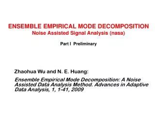
ENSEMBLE EMPIRICAL MODE DECOMPOSITION Noise Assisted Signal Analysis (nasa) Part I Preliminary. Zhaohua Wu and N. E. Huang: Ensemble Empirical Mode Decomposition: A Noise Assisted Data Analysis Method. Advances in Adaptive Data Analysis, 1, 1-41, 2009. Theoretical Foundations.

E N D
ENSEMBLE EMPIRICAL MODE DECOMPOSITIONNoise Assisted Signal Analysis (nasa) Part I Preliminary Zhaohua Wu and N. E. Huang: Ensemble Empirical Mode Decomposition: A Noise Assisted Data Analysis Method. Advances in Adaptive Data Analysis, 1, 1-41, 2009
Theoretical Foundations • Intermittency test, though ameliorates the mode mixing, destroys the adaptive nature of EMD. • The EMD study of white noise guarantees a uniformed frame of scales. • The cancellation of white noise with sufficient number of ensemble.
Theoretical Background I Intermittency
Sifting with Intermittence Test • To avoid mode mixing, we have to institute a special criterion to separate oscillation of different time scales into different IMF components. • The criteria is to select time scale so that oscillations with time scale longer than this pre-selected criterion is not included in the IMF.
Observations • Intermittency test ameliorates the mode mixing considerably. • Intermittency test requires a set of subjective criteria. • EMD with intermittency is no longer totally adaptive. • For complicated data, the subjective criteria are hard, or impossible, to determine.
Effects of EMD (Sifting) • To separate data into components of similar scale. • To eliminate ridding waves. • To make the results symmetric with respect to the x-axis and the amplitude more even. • Note: The first two are necessary for valid IMF, the last effect actually cause the IMF to lost its intrinsic properties.
Theoretical Background II A Study of White Noise
Wu, Zhaohua and N. E. Huang, 2004: A Study of the Characteristics of White Noise Using the Empirical Mode Decomposition Method, Proceedings of the Royal Society of London , A 460, 1597-1611.
Methodology • Based on observations from Monte Carlo numerical experiments on 1 million white noise data points. • All IMF generated by 10 siftings. • Fourier spectra based on 200 realizations of 4,000 data points sections. • Probability density based on 50,000 data points data sections.
IMF 1 2 3 4 5 6 7 8 9 number of peaks 347042 168176 83456 41632 20877 10471 5290 2658 1348 Mean period 2.881 5.946 11.98 24.02 47.90 95.50 189.0 376.2 741.8 period in year 0.240 0.496 0.998 2.000 3.992 7.958 15.75 31.35 61.75 IMF Period Statistics
Empirical Observations : IINormalized spectral area is constant
Empirical Observations : IIINormalized spectral area is constant
Empirical Observations : IIIThe product of the mean energy and period is constant
Empirical Observation: Histograms IMFs By Central Limit theory IMF should be normally distributed.
Fundamental Theorem of Probability • If we know the density function of a random variable, x, then we can express the density function of any random variable, y, for a given y=g(x). The procedure is as follows:
Fundamental Theorem of Probability • If we know the density function of a random variable, x, is normal, then x-square should be
DEGREE OF FREEDOM • Random samples of length N contains N degree of freedom • Each Fourier component contains one degree of freedom • For EMD, the shares of DOF is proportional to its share of energy; therefore, the degree of freedom for each IMF is given as
CHI SQUARE-DISTRIBUTION OF ENERGY chi-square dist.
Formula of Confidence Limit for IMF Distributions IV For a Gaussian distribution, it is often to relate α to the standard deviation, σ , i.e., α confidence level corresponds to k σ, where k varies with α. For example, having values -2.326, -0.675, -0.0, 0.675, and 2.326 for the first, 25th, 50th, 75th and 99th percentiles (with α being 0.01, 0.25, 0.5, 0.75, 0.99), respectively.
1 mon 1 yr 10 yr 100 yr Statistical Significance for SOI IMFs IMF 4, 5, 6 and 7 are 99% statistical significance signals.
Summary • Not all IMF have the same statistical significance. • Based on the white noise study, we have established a method to determine the statistical significant components. • References: • Wu, Zhaohua and N. E. Huang, 2003: A Study of the Characteristics of White Noise Using the Empirical Mode Decomposition Method, Proceedings of the Royal Society of London A460, 1597-1611. • Flandrin, P., G. Rilling, and P. Gonçalvès, 2003: Empirical Mode Decomposition as a Filterbank, IEEE Signal Proc Lett. 11 (2): 112-114.
Observations The white noise signal consists of signal of all scales. EMD separates the scale dyadically. The white noise provide a uniformly distributed frame of scales through EMD.
Flandrin, P., G. Rilling and P. Goncalves, 2004: Empirical Mode Decomposition as a filter bank. IEEE Signal Process. Lett., 11, 112-114.Flandrin, P., P. Goncalves and G. Rilling, 2005: EMD equivalent filter banks, from interpretation to applications.Introduction to Hilbert-Huang Transform and its Applications, Ed. N. E. Huang and S. S. P. Shen, p. 57-74. World Scientific, New Jersey, Different Approaches but reach the same end.
Theoretical Background III Effects of adding White Noise
Some Preliminary • Robert John Gledhill, 2003: Methods for Investigating Conformational Change in Biomolecular Simulations, University of Southampton, Department of Chemistry, Ph D Thesis. • He investigated the effect of added noise as a tool for checking the stability of EMD.
Some Preliminary • His basic assumption is that the correct result is the one without noise:
Test results Top Whole data perturbed; bottom only 10% perturbed. 10%