Medical imaging
Medical imaging. Sound waves - Ultrasound Using the Electromagnetic Spectrum Visible light - Fluorescence X-ray , Fluoroscopy, CT, & Angiography gamma rays - PET (positron emission tomography) Radio waves from nuclear spin – MRI. Visible - interlude.

Medical imaging
E N D
Presentation Transcript
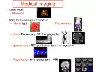
Medical imaging • Sound waves • - Ultrasound • Using the Electromagnetic Spectrum • Visible light - Fluorescence • X-ray, Fluoroscopy, CT, & Angiography • gamma rays - PET (positron emission tomography) • Radio waves from nuclear spin – MRI
Visible - interlude Electromagnetic Spectrum
Visible microscope Endoscopy • Versatile and inexpensive • Extensive Histology • Diffraction limits resolution to approximately 0.2 micrometers. • Only image dark or strongly refracting objects effectively • (staining however can distinguish • different tissue types – kill and fix) Laparoscopy - ovary
Visible Luminescence – e- absorb energy (mech, chem, & EM) and then emit light photoluminescence – ultraviolet or visible excitation fluorescence (fast) & phosphorescence (slow) – absorb light and then reemit at lower energy (longer wavelength) http://zeiss-campus.magnet.fsu.edu/articles/basics/fluorescence.html
Visible fluorescence (fast) & phosphorescence (slow) Prostate tumor Fluorescence UK T2 MRI – UK 7T http://www.activemotif.com Antibody – fluorescence – single laser excitation - nucleus
Primed Frame Z axis recovering longitudinal magnetization (T1) remaining transverse magnetization (time constant T2(*))
Z axis T1 (recovery) and …………. time time ..… T2 (dephasing) together.
Back to MRI Understanding Inversion Recovery Gradient Echo to measure T1 And Spin Echo to measure T2
Model of Head Coil Excite Listen RF (90 degrees) B0
Inversion Recovery Gradient Echo to measure T1 – your book – on single voxel Mz = -M0+ 2M0[1-exp (-t/T1)] 180 excitation z’ After time τ rotate 90 and “listen immediately” τ3 end - listen y’ τ2 x’ τ1 start τ1 z’ z’ Signal Magnitude = |Mz |= |-M0+ 2M0[1-exp (- τ /T1)]| Signal Magnitude start τ3 y’ end τ2 start y’ end listen x’ x’ τ τ2 τ1 τ3
Spin Echo to measure T2 – on single voxel Experiment repeated over and over again with different t’s (your book uses this symbol τ in section 4.2.5 and equation (4.32). The 180 degree flip allows for spin in static (constant in time) magnetic fields to “fix” their dephasing (T2’). Residual signal decay (loss) is due to T2 only. http://en.wikipedia.org/wiki/Spin_echo
Spin Echo to measure T2 – from you book - on single voxel 180 90 My’ =
end start Collective Magnetic Moment of Protons MRI excite with slice selection Body Coil - Gradients Radio Waves 123 MHz B0
excite 3.1 T 127 MHz 3.0 T 123 MHz 2.9 T 119 MHz ƋBz/ƋBz = Gz Apply Z gradient Picture of graph Got one of the 3 orthogonal spatial dimensions when we excite. Z gradient on
excite 119 MHz 123 MHz 127 MHz Phase difference in z direction Within the slice BAD (but we can fix) FT Slice Thickness
Model of Head Coil Then we could just LISTEN B0 TurnZ gradient off. Turn RF off. Signal come only from protons in slice. One dimension down … two to go.
Image should be Image we get of water container
better to LISTEN like this Model of Head Coil 3.1 T 127 MHz precess fast 3.0 T 123 MHz precess regular ƋBx/ ƋBx = Gx Apply X gradient precess slow 2.9 T 119 MHz Got second of the 3 orthogonal spatial dimensions when we listen. X gradient on
Image should be Image we get of water container
phase encode (after we excite before we listen) Model of Head Coil fast 3.1 T 127 MHz regular 3.0 T 123 MHz Acquired phase due to gradient 2.9 T 119 MHz slow Get 3rd spatial dimension with phase encoding. Short pulse of Y gradient in this example. This leads repeating the entire process (aka the “TR”) for each voxel in the phase encoding direction (y here).
Image should be Image we get of water container
Spin Echo ……. and repeat for each pixel in the phase encoding direction // TR Siemens
Gradient Echo axial slice excite Slice select gradient fix phases z ……. and repeat for each pixel in the phase (y-axis) encoding direction y x TE // TR Siemens
Excite (RF) 3.1 T 127 MHz 3.0 T 123 MHz 2.9 T 119 MHz ƋBz/ƋBz = Gz Apply Z gradient Picture of graph Got one of the 3 orthogonal spatial dimensions when we excite. Z gradient on
Fix phases 3.0 T 123 MHz 2.9 T 119 MHz 3.1 T 127 MHz ƋBz/ƋBz = Gz Apply Z gradient Picture of graph Within the glass of water, these protons had extra phase Within the glass of water, these protons had too little phase
Gradient Echo axial slice z Phase encode to spatially locate magnetic moments in the y direction y x // TR Siemens
phase encode (after we excite before we listen) Model of Head Coil fast 3.1 T 127 MHz regular 3.0 T 123 MHz slow 2.9 T 119 MHz Short pulse of Y gradient in this example. This leads repeating the entire process (aka the “TR”) for each voxel in the phase encoding direction (y here).
Gradient Echo axial slice Readout gradient – can locate voxels based on their precessional frequency z y ADC – analog to digital converter (“listens” 256 times in rapid succession if 256 pixels in x direction) (little lie … we really listen 1024 time to avoid wrapping) x Preparation for readout gradient so phases are not wrong // TR
Model of Head Coil Preparation for readout gradient precess slow 2.9 T 119 MHz 3.0 T 123 MHz precess regular ƋBx/ ƋBx = Gx Apply X gradient 3.1 T 127 MHz precess fast X gradient on
LISTEN ADC on Model of Head Coil 3.1 T 127 MHz precess fast 3.0 T 123 MHz precess regular ƋBx/ ƋBx = Gx Apply X gradient precess slow 2.9 T 119 MHz X gradient on
Spin Echo …… repeat // TR Same idea, but we have the 180 degree flip to fix T2’ (magnetic field variations that are constant in time) Siemens
MR Signal MR Signal T2 Decay T1 Recovery 1 s 50 ms Allen W. Song Duke University
Proton Density Contrast • Technique: use very long time between RF shots (large TR) and very short delay between excitation and readout window (short TE) • Useful for anatomical reference scans • Several minutes to acquire 256256128 volume • ~1 mm resolution
MR Signal MR Signal T2 Decay T1 Recovery Proton Density Contrast 1 s 50 ms
T2* and T2 Contrast • Technique: use largeTR and intermediateTE • Useful for anatomical and functional studies • Several minutes for 256x256X128 volumes, or ~several seconds to acquire 646420 volume • 1mm resolution for anatomical scans or 4 mm resolution [better is possible with better gradient system, and a little longer time per volume]
MR Signal MR Signal T2 Decay T1 Recovery T2* and T2 Contrast 1 s 50 ms
Long TR and vary TE (echo time = listen time) effectively a proton density nice T2 contrast most of signal gone
T1 Contrast • Technique: use intermediate timing between RF shots (intermediate TR) and very short TE, also use large flip angles • Useful for anatomical reference scans • Several minutes to acquire 256256128 volume • ~1 mm resolution
MR Signal MR Signal T2 Decay T1 Recovery T1 Contrast 1 s 50 ms