Download
1 / 51
530 likes | 899 Views
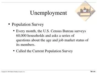
U . L. u = x 100%. Unemployment. Unemployment rate The Current Population Survey is a joint project of the BLS and the Bureau of the Census Every month, 1,600 CPS interviewers survey 60,000 households to establish job market status of each member of the household.

E N D
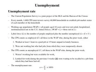
U . L u = x 100% Unemployment Unemployment rate • The Current Population Survey is a joint project of the BLS and the Bureau of the Census • Every month, 1,600 CPS interviewers survey 60,000 households to establish job market status of each member of the household. • Working-age population (WAP) = all people aged 16 years and over not jailed, hospitalized, institutionalized nor in the U.S. Armed Forces. (WAP = L + those not in L) • Labor force (L) is the number of people employed plus the number unemployed (L=E+U ). • The CPS counts as employed (E ) all those in the WAP who, during the prior week, either • Worked at least 1 hour in a paid job or 15 hours unpaid in family business. • Were not working but who had jobs from which they were temporarily absent. • The CPS counts as unemployed (U ) all those in the WAP who, during the prior week, • Weren’t working but were available for work, • Looked for work during the previous 4 weeks ORwere waiting to be recalled to a job from which they had been laid off. • The unemployment rate:
= Unemployment Types of unemployment • Frictional (uf ): workers temporarily between jobs because of a move/career change. • Structural (us ): workers displaced by automation. • Cyclical (uc ): workers who loose their jobs due to recession. u = uf + us + uc • Natural rate of unemployment (un ≈ 5%):It’s the rate at which inflation remains constant. uf + us = 5% uc = 0.81%
30 25 20 15 Unemployment Rate 10 5 0 1890 1900 1910 1920 1930 1940 1950 1960 1970 1980 1990 2000 2010 Year Unemployment 1900 to 2010 2011 researchstlouisfedorg UNRATE
Alternate measures of unemployment Unemployed workers who have actively looked for work for 4 weeks Discouraged workers are unemployed and have stopped looking for workbecause they think no work is available for them Other marginally attached workers are unemployed, would like, and ableto work but have not looked for work recently Underemployed are PT workers who want to work FT but cannot due to economic reasons u1 = % of LF unemployed 15 weeks or longer u2 = % of LF who lost jobs or completed temporary work u3 = official unemployment rate u4 = u3 + discouraged workers u5 = u4 + Other marginally attached workers u6 = u5 + underemployed
Alternate measures of unemployment 1994-2010 u6 u5 u3 u4 UNRATE, U4RATE, U5RATE, U6RATE
Unemployment Rates by Race/Ethnicity 1973-2010 Black Hispanic White Asian LNS14000006, LNS14000003 LNU04032183, LNS14000009
Unemployment Rates by Gender 1960-2010 Male Female 2011 researchstlouisfedorg USALFFEMADSMEI, USAEMPFEMADSMEI, USALFMALEADSMEI, USAEMPMALADSMEI
Unemployment Rates by Education 1992-2010 HS dropout HS no college Some college or Assoc Degree Bachelor’s Degree or higher LNS14027662, LNS14027689 LNS14027660, LNS14027659
Unemployment Rates by Age1970-2010 Teenagers 20-24 year olds Adults USAURANAA, USAUR24NAA, USAURTNAA
Unemployment rate and average duration1948 to 2010 Avg Duration of unemployment Unemployment UNRATE UEMPMEAN
Unemployment Rates by Industry 2001-2011 Source: www.bls.gov
Unemployment Rates by Industry 2001-2011 Source: www.bls.gov
Unemployed Persons by Duration of Unemployment, 1948-2002 • Although most spells of unemployment do not last very long, most weeks of unemployment can be attributed to workers who are in very long spells
Flows Between Employment and Unemployment Job Losers ( pE ) Employed (E workers) Unemployed (U Workers) Job Finders ( qU ) Suppose a person is either working or unemployed. At any point in time, some workers lose their jobs and unemployed workers find jobs. If the probability of losing a job equals p, there are pE job losers. If the probability of finding a job equals q, there are qU job finders.
Dynamic Flows in the US Labor Market, May 1993 1.8 million Unemployed: 8.9 million Employed: 119.2 million 2.0 million 3.2 million 1.7 million 1.5 million 3.0 million Out of Labor Force: 65.2 million
Job Search • The asking wage makes the worker indifferent between continuing his search activities and accepting the job offer at hand • An increase in the benefits from search raises the asking wage and lengthens the duration of the unemployment spell • An increase in search costs reduces the asking wage and shortens the duration of the unemployment spell
The Wage Offer Distribution Frequency $5 $8 $22 $25 Wage The wage offer distribution gives the frequency distribution of potential job offers A given worker can get a job paying anywhere from $5 to $25 per hour What is the probability that the worker receives a wage offer between 5 and $8?
The Asking Wage The marginal cost curve gives the cost of an additional search. It is upward sloping because the better the job offer at hand, the greater the opportunity cost of an additional search. Dollars MC MR$10 MC$20 The marginal revenue curve gives the gain from an additional search. It is downward sloping because the better the offer at hand, the less there is to gain from an additional search . MC$15 = MR$15 MC$10 MR$20 MR 0 $15 $10 $20 Wage Offer at Hand The asking wage equates the marginal revenue and the marginal cost of search
The Asking Wage Dollars MC0 MC MC1 MR0 MR1 MR Wage Wage 15 10 10 15 People with higher discount rates are more worried about the present than their futures So they have little to gain from additional searches UI benefits reduce the cost of searching for the right job So there is much to gain from additional searches
The Asking Wage Dollars MC0 MC1 MR Wage 10 15 • The internet can greatly reduce the costs associated with job search. • Kuhn and Skuterud (2004): • D-in-D estimates: people using the Internet found work 0.3 months faster • (perhaps because the Internet helps secure a high w offer quicker) • This result vanishes in a regression that controls educational attainment, gender, and age. • Why? The Internet is ineffective, used to meet UI job search requirements, or used by people who do not put in the time and effort to find work (selection bias).
The Relationship Between the Probability of Finding a New Job and UI Benefits .08 .06 .04 .02 .00 • Before the 2008 recession, UI ended at 26 weeks. • The probability of finding a new job spikes when UI benefits are exhausted • The probability of finding a new job spikes again at 15 weeks after benefits are exhausted US increased UI benefits from 26 to 99 weeks 1 6 11 16 21 26 31 36 41 46 51 56 61 66 71 76 81 86 91 96 101 (Weeks of UI benefits) • Hence, UI benefits should lengthen the duration of unemployment spells
Funding the UI System: Imperfect Experience Rating Tax rate 5.4% 0.1% 0 l1 l0 Firm layoff Rate in the Past UI is funded by payroll tax on employers—the more lay offs the higher the tax The state determines up to what level to tax payrolls In California, the first $7000 paid to employees is taxed at a rate of between 0.1% to 5.4%
Funding the UI System: Imperfect Experience Rating Tax rate 5.4% 0.1% 0 l1 l l0 Firm layoff Rate in the Past If the firm has a layoff rate less than l0, for each employee, the firm pays a tax to the Federal UI fund equal to the lesser of (0.1%)(wh) (0.1%)($7000) or
Funding the UI System: Imperfect Experience Rating Tax rate 5.4% t 0.1% 0 l1 l0 l Firm layoff Rate in the Past If the firm has a layoff rate between l0 and l1, for each employee, the firm pays a tax to the Federal UI fund equal to the lesser of (t)(wh) (t)($7000) or
Funding the UI System: Imperfect Experience Rating Tax rate 5.4% 0.1% 0 l1 l0 l Firm layoff Rate in the Past If the firm has a layoff rate greater than l1, for each employee, the firm pays a tax to the Federal UI fund equal to the lesser of (5.4%)(wh) (5.4%)($7000) Hence, firms with high layoff rates are subject to perfect experience rating, meaning firms with low layoff rates subsidize firms with high layoff rates or
Efficiency Wages and Unemployment The shirking model • If workers are equally productive in a perfectly competitive labor market, they get paid w* whether they • work productively (which is costly) • goof off or make long distance phone calls at work (shirk) • Workers may shirk after they are hired because • their incentives are not perfectly aligned with the owner’s (principal-agent) • information about their performance is limited (asymmetric information) • getting fired after being caught doesn’t prevent them from working for someone else making w* (moral hazard) • Solutions: • Increased monitoring (costly and not perfect) • Bonding (e.g., employee don’t get student loans paid off if they quit early) • Piece rate pay (brownnosers lobby supervisors for the ‘best’ working conditions) • Paying wage wNS that exceeds w* (efficiency wage), which makes being fired costly (Dw = wNS – w*)
The Determination of the Efficiency Wage Dollars S w0 w* D Employment E0 N U If shirking is not a problem, the market clears at wage w*. Shirking may occur because fired workers can find work somewhere else making w*. At high unemployment (N – E0), workers toe the line at a slightly higher wage w0 because high unemployment attracts workers who will not shirk at w0.
The Determination of the Efficiency Wage Dollars SNS S w1 w0 w* D Employment E0 E1 N U At low unemployment (N – E1) firms have to pay much more to inhibit shirking Hence the no-shirking supply curve is upward sloping, and asymptotically approaches S.
The Determination of the Efficiency Wage Dollars SNS S wNS w* D Employment ENS N The efficient wage model suggests that some unemployment is necessary to keep employees in line (structural unemployment) Efficiency wage wNS is given by the intersection of the no-shirking supply curve and demand curve
wNS 0 w* 0 The Determination of the Efficiency Wage and Economic Contraction Dollars SNS S wNS 1 D0 D1 w* 1 E1 E0 N Employment A fall in output demand reduces labor demand, reducing the competitive wage. If firms pay an efficiency wage, the contraction also reduces the efficiency wage Efficiency wage theory suggests that wages are stickybecause the decline in wNS is much smaller than the fall in w*.
wNS The Determination of the Efficiency Wage and UI Benefits Dollars SNS S D w* E N Employment • An increase in UI benefits decreases no-shirking labor supply • the wage needed to inhibit shirking (wNS) • Unemployment (N – E) • The cost of getting caught shirking (wNS – w*) and increases
wNS wNS 1 0 The Wage Curve: The Relation Between Wage Levels and Unemployment Across Regions Wage Unemployment Rate u1 u0 Efficiency wages may play an important role in unemployment Geographic regions that offer higher wage rates also tend to have lower unemployment rates Hence, the greater is the surplus of workers (u), the lower the wage??? Yes if shirking is problematic
AS The Phillips Curve Recessionary Gap • A recessionary gap occurs when GDP is less than potential GDP. • Resources, capital, and workers are not being fully utilized, and so u is high. • As a result, there is downward pressure on wages… • ….prices fall Note: Unemployment insurance replaces a portion of a newly unemployed worker’s income. Designed to prevent the “next” Great Depression. PL PL AD GDP YFE
AS The Phillips Curve Inflationary Gap • An inflationary gap occurs when GDP exceeds potential GDP. • Workers are working overtime and firms are competing for their labor, resulting in low u • As a result, there is upward pressure on wages… • ….prices fall PL PL AD GDP YFE
The Phillips Curve The business cycle • The figure shows recent cycles in real GDP. • Recessions began in mid-1990 and in first quarter of 2001. • The longest expansion in U.S. history ran from the March 1991 to March 2001. • When GDP decreases The unemployment rate increases And a little later, the inflation rate decreases • As real GDP increases toward potential GDP, unemployment falls toward its natural rate, which leads to an eventual rise in inflation.
The Phillips Curve Source:http://wwwblsgov/ The Phillips curve describes the negative correlation between the inflation rate and the unemployment rate The curve implies that an economy faces a trade-off between inflation and unemployment
(1961-2005) The Phillips Curve What happened? Inflation expectations were changing
Expected Inflation The Phillips Curve • The yields on two different kinds of Treasury securities are used to calculate a measure of inflation expectations: • nominal treasury notes • treasury inflation-protected securities (TIPS) • Their difference is called the TIPS spread • Because the market's expectations for inflation are priced TIPS, the measure that is derived from the yields is a good estimate of the market's estimate of future inflation • The calculation involves correcting for some biases: • inflation-risk premium • liquidity premium
Expected Inflation The Phillips Curve • The liquidity premium (LP): difference between the yields on 10-year on-the-run and off-the-run treasury notes • Spread (or bias) is equal to the difference between inflation expectations from the Survey of Professional Forecasters (SPF) and the TIPS-derived expected inflation (TIPS) • Regressing spread (or bias) on LP and LP2 gives predicted bias: bias = a + b1∙LP + b2∙LP2 • Subtracting this from TIPS-derived expected inflation yields an unbiased estimate of expected inflation: pe = TIPS – bias(LP) picks up the bias due to inflation risk picks up the bias due to liquidity
The Phillips Curve Rate of Inflation Long Run 0 Short Run Unemployment Rate 5 The economy is initially at the point where there is no inflationand a 5 percent unemployment rate
The Phillips Curve Rate of Inflation Long Run 7 0 Short Run Unemployment Rate 3 5 If monetary policy increases the inflation rate to 7 percent, job searchers will suddenly find many jobs that meet their reservation wage and the unemployment rate falls in the short run
The Phillips Curve Rate of Inflation Long Run 7 0 Short Run Unemployment Rate 3 5 In the long run, the unemployment rate is still 5 percent, but there is now a higher rate of inflation Over time, workers realize that the inflation rate is higher and will adjust their reservation wage upward, returning the economy to having u= 5% and p = 7 In the long run, therefore, there is no trade-off between inflation and unemployment
(1975-2005) The Augmented Phillips Curve m is the markup of firm’s unit price over unit cost x is all other variables affecting wage setting q is positive (but if q = 0, Phillips curve) More stringent antitrust legislation decreases market power Increasing UI benefits NAIRU or Natural Rate of unemployment NAIRU increases NAIRU decreases Source:http://wwwblsgov/
Unemployment and Interest Rates 1954-2011 The unemployment rate lags the federal funds rate bya couple of years ?
Unemployment and Interest Rates 1987-2011 u
Unemployment and Interest Rates 1989-2008 u Fed Funds Rate
Unemployment and Interest Rates 1989-2008 u Fed Funds Rate (lagged one year)
Unemployment and Interest Rates 1989-2008 u Fed Funds Rate (lagged two years)