Download
1 / 31
540 likes | 1.74k Views
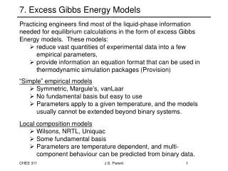
7. Excess Gibbs Energy Models. Practicing engineers find most of the liquid-phase information needed for equilibrium calculations in the form of excess Gibbs Energy models. These models: reduce vast quantities of experimental data into a few empirical parameters,

E N D
7. Excess Gibbs Energy Models • Practicing engineers find most of the liquid-phase information needed for equilibrium calculations in the form of excess Gibbs Energy models. These models: • reduce vast quantities of experimental data into a few empirical parameters, • provide information an equation format that can be used in thermodynamic simulation packages (Provision) • “Simple” empirical models • Symmetric, Margule’s, vanLaar • No fundamental basis but easy to use • Parameters apply to a given temperature, and the models usually cannot be extended beyond binary systems. • Local composition models • Wilsons, NRTL, Uniquac • Some fundamental basis • Parameters are temperature dependent, and multi-component behaviour can be predicted from binary data. J.S. Parent
Excess Gibbs Energy Models • Our objectives are to learn how to fit Excess Gibbs Energy models to experimental data, and to learn how to use these models to calculate activity coefficients. J.S. Parent
Margule’s Equations • While the simplest Redlich/Kister-type expansion is the Symmetric Equation, a more accurate model is the Margule’s expression: • (11.7a) • Note that as x1 goes to zero, • and from L’hopital’s rule we know: • therefore, • and similarly J.S. Parent
Margule’s Equations • If you have Margule’s parameters, the activity coefficients are easily derived from the excess Gibbs energy expression: • (11.7a) • to yield: • (11.8ab) • These empirical equations are widely used to describe binary solutions. A knowledge of A12 and A21 at the given T is all we require to calculate activity coefficients for a given solution composition. J.S. Parent
van Laar Equations • Another two-parameter excess Gibbs energy model is developed from an expansion of (RTx1x2)/GE instead of GE/RTx1x2. The end results are: • (11.13) • for the excess Gibbs energy and: • (11.14) • (11.15) • for the activity coefficients. • Note that: as x10, ln1 A’12 • and as x2 0, ln2 A’21 J.S. Parent
Local Composition Models • Unfortunately, the previous approach cannot be extended to systems of 3 or more components. For these cases, local composition models are used to represent multi-component systems. • Wilson’s Theory • Non-Random-Two-Liquid Theory (NRTL) • Universal Quasichemical Theory (Uniquac) • While more complex, these models have two advantages: • the model parameters are temperature dependent • the activity coefficients of species in multi-component liquids can be calculated from binary data. • A,B,C A,B A,C B,C • tertiary mixture binary binary binary J.S. Parent
Wilson’s Equations for Binary Solution Activity • A versatile and reasonably accurate model of excess Gibbs Energy was developed by Wilson in 1964. For a binary system, GE is provided by: • (11.16) • where • (11.24) • Vi is the molar volume at T of the pure component i. • aij is determined from experimental data. • The notation varies greatly between publications. This includes, • a12 = (12 - 11), a12 = (21 - 22) that you will encounter in Holmes, M.J. and M.V. Winkle (1970) Ind. Eng. Chem.62, 21-21. J.S. Parent
Wilson’s Equations for Binary Solution Activity • Activity coefficients are derived from the excess Gibbs energy using the definition of a partial molar property: • When applied to equation 11.16, we obtain: • (11.17) • (11.18) J.S. Parent
Wilson’s Equations for Multi-Component Mixtures • The strength of Wilson’s approach resides in its ability to describe multi-component (3+) mixtures using binary data. • Experimental data of the mixture of interest (ie. acetone, ethanol, benzene) is not required • We only need data (or parameters) for acetone-ethanol, acetone-benzene and ethanol-benzene mixtures • The excess Gibbs energy is written: • (11.22) • and the activity coefficients become: • (11.23) • where ij = 1 for i=j. Summations are over all species. J.S. Parent
Wilson’s Equations for 3-Component Mixtures • For three component systems, activity coefficients can be calculated from the following relationship: • Model coefficients are defined as (ij = 1 for i=j): J.S. Parent
Comparison of Liquid Solution Models Activity coefficients of 2-methyl-2-butene + n-methylpyrollidone. Comparison of experimental values with those obtained from several equations whose parameters are found from the infinite-dilution activity coefficients. (1) Experimental data. (2) Margules equation. (3) van Laar equation. (4) Scatchard-Hamer equation. (5) Wilson equation. J.S. Parent
8. Non-Ideal VLE to Moderate Pressure 12.4 text • We now have the tools required to describe and calculate vapour-liquid equilibrium conditions for even the most non-ideal systems. • 1. Equilibrium Criteria: • In terms of chemical potential • In terms of mixture fugacity • 2. Fugacity of a component in a non-ideal gas mixture: • 3. Fugacity of a component in a non-ideal liquid mixture: J.S. Parent
g, f Formulation of VLE Problems • To this point, Raoult’s Law was only description we had for VLE behaviour: • We have repeatedly observed that calculations based on Raoult’s Law do not predict actual phase behaviour due to over-simplifying assumptions. • Accurate treatment of non-ideal phase equilibrium requires the use of mixture fugacities. At equilibrium, the fugacity of each component is the same in all phases. Therefore, • or, • determines the VLE behaviour of non-ideal systems where Raoult’s Law fails. J.S. Parent
Non-Ideal VLE to Moderate Pressures • A simpler expression for non-ideal VLE is created upon defining a lumped parameter, F. • 12.2 • The final expression becomes, • (i = 1,2,3,…,N) 12.1 • To perform VLE calculations we therefore require vapour pressure data (Pisat), vapour mixture and pure component fugacity correlations (i) and liquid phase activity coefficients (i). J.S. Parent
Non-Ideal VLE to Moderate Pressures • Sources of Data: • 1. Vapour pressure: Antoine’s Equation (or similar correlations) • 12.3 • 2. Vapour Fugacity Coefficients: Viral EOS (or others) • 12.6 • 3. Liquid Activity Coefficients • Binary Systems - Margule, van Laar, Wilson, NRTL, Uniquac • Ternary (or higher) Systems - Wilson, NRTL, Uniquac J.S. Parent
Non-Ideal VLE Calculations • The Pxy diagram to the right • is for the non-ideal system of • chloroform-dioxane. • Note the P-x1 line represents • a saturated liquid, and is commonly BUBL LINE • referred to as the bubble-line. • P-y1 represents a saturated • vapour, and is referred to as the • dew line (the point where a liquid DEW LINE • phase is incipient). J.S. Parent
Non-Ideal BUBL P Calculations • The simplest VLE calculation of the five is the bubble-point pressure calculation. • Given: T, x1, x2,…, xn Calculate P, y1, y2,…, yn • To find P, we start with a material balance on the vapour phase: • Our equilibrium relationship provides: • 12.9 from 12.1 • which yields the Bubble Line equation when substituted into the material balance: • or • 12.11 J.S. Parent
Non-Ideal BUBL P Calculations • Non-ideal BUBL P calculations are complicated by the dependence of our coefficients on pressure and composition. • Given: T, x1, x2,…, xn Calculate P, y1, y2,…, yn • To apply the Bubble Line Equation: • requires: • ? • • • Therefore, the procedure is: • calculate Pisat, and i from the information provided • assume i=1, calculate an approximate PBUBL • use this estimate to calculate an approximate i • repeat PBUBL and i calculations until solution converges. J.S. Parent
Non-Ideal Dew P Calculations • The dew point pressure of a vapour is that pressure which the mixture generates an infinitesimal amount of liquid. The basic calculation is: • Given: T, y1, y2,…, yn Calculate P, x1, x2,…, xn • To solve for P, we use a material balance on the liquid phase: • Our equilibrium relationship provides: • 12.10 from 12.1 • From which the Dew Line expression needed to calculate P is generated: • 12.12 J.S. Parent
Non-Ideal Dew P Calculations • In trying to solve this equation, we encounter difficulties in estimating thermodynamic parameters. • Given: T, y1, y2,…, yn Calculate P, x1, x2,…, xn • ? • ? • • While the vapour pressures can be calculated, the unknown pressure is required to calculate i, and the liquid composition is needed to determine i • Assume both parameters equal one as a first estimate, calculate P and xi • Using these estimates, calculate i • Refine the estimate of xi (12.10) and estimate i • Refine the estimate of P • Iterate until pressure and composition converges. J.S. Parent
8. Non-Ideal Bubble and Dew T Calculations • The Txy diagram to the right • is for the non-ideal system of • ethanol(1)/toluene(2) at P =1atm. • Note the T-x1 line represents • a saturated liquid, and is commonly DEW LINE • referred to as the bubble-line. • T-y1 represents a saturated • vapour, and is referred to as the • dew line (the point where a liquid • phase is incipient). • BUBL LINE J.S. Parent
Non-Ideal BUBL T Calculations • Bubble point temperature calculations are among the more complicated VLE problems: • Given: P, x1, x2,…, xn Calculate T, y1, y2,…, yn • To solve problems of this sort, we use the Bubble Line equation: • 12.11 • The difficulty in determining non-ideal bubble temperatures is in calculating the thermodynamic properties Pisat, i, and i. • Since we have no knowledge of the temperature, none of these properties can be determined before seeking an iterative solution. J.S. Parent
Non-Ideal BUBL T Calculations: Procedure • 1. Estimate the BUBL T • Use Antoine’s equation to calculate the saturation temperature (Tisat) for each component at the given pressure: • Use TBUBL = xi Tisat as a starting point • 2. Using this estimated temperature and xi’s calculate • Pisat from Antoine’s equation • Activity coefficients from an Excess Gibbs Energy Model (Margule’s, Wilson’s, NRTL) • Note that these values are approximate, as we are using a crude temperature estimate. J.S. Parent
Non-Ideal BUBL T Calculations: Procedure • 3. Estimate i for each component. • We now have estimates of T, Pisatand i, but no knowledge of i. • Assume that i=1 and calculate yi’s using: 12.9 • Plug P, T, and the estimates of yi’s into your fugacity coefficient expression to estimate i. • Substitute thesei estimates into 12.9 to recalculate yi and continue this procedure until the problem converges. • Step 3 provides an estimate of i that is based on the best T, Pisat, i, and xi data that is available at this stage of the calculation. • If you assume that the vapour phase is a perfect gas mixture, all i =1. J.S. Parent
Non-Ideal BUBL T Calculations: Procedure • 4. Our goal is to find the temperature that satisfies our bubble point equation: • (12.11) • Our estimates of T, Pisat, i and i, are approximate since they are based on a crude temperature estimate (T = xi Tisat) • Calculate P using the Bubble Line equation (12.11) • If Pcalc < Pgiven then increase T • If Pcalc > Pgiven then decrease T • If Pcalc = Pgiven then T = TBUBL • The simplest method of finding TBUBL is a trial and error method using a spreadsheet. • Follow steps 1 to 4 to find Pcalc. • Change T and repeat steps 2, 3, and 4 until Pcalc = Pgiven J.S. Parent
Non-Ideal DEW T Calculations • The dew point temperature of a vapour is that which generates an infinitesimal amount of liquid. • Given: P, y1, y2,…, yn Calculate T, x1, x2,…, xn • To solve these problems, use the Dew Line equation: • 12.12 • Once again, we haven’t sufficient information to calculate the required thermodynamic parameters. • Without T and xi’s, we cannot determine i, i or Pisat. J.S. Parent
Non-Ideal DEW T Calculations: Procedure • 1. Estimate the DEW T • Using P, calculate Tisat from Antoine’s equation • Calculate T = yi Tisat as a starting point • 2. Using this temperature estimate and yi’s, calculate • Pisat from Antoine’s equation • i using the virial equation of state • Note that these values are approximate, as we are using a crude temperature estimate. J.S. Parent
Non-Ideal DEW T Calculations: Procedure • 3. Estimate i, for each component • Without liquid composition data, you cannot calculate activity coefficients using excess Gibbs energy models. • A. Set i=1 • B. Calculate the Dew Pressure: • C. Calculate xi estimates from the equilibrium relationship: • D. Plug P,T, and these xi’s into your activity coefficient model to estimate i for each component. • E. Substitute these i estimates back into 12.12 and repeat B through D until the problem converges. J.S. Parent
Non-Ideal DEW T Calculations: Procedure • 4. Our goal is to find the temperature that satisfies our Dew Line equation: • (12.12) • Our estimates of T, Pisat, i and i, are based on an approximate temperature (T = xi Tisat) we know is incorrect. • Calculate P using the Bubble Line equation (12.11) • If Pcalc < Pgiven then increase T • If Pcalc > Pgiven then decrease T • If Pcalc = Pgiven then T = TDew • The simplest method of finding TDew is a trial and error method using a spreadsheet. • Follow steps 1 to 4 to find Pcalc. • Change T and repeat steps 2, 3, and 4 until Pcalc = Pgiven J.S. Parent
9.3 Modified Raoult’s Law • At low to moderate pressures, the vapour-liquid equilibrium equation can be simplified considerably. • Consider the vapour phase coefficient, i: • Taking the Poynting factor as one, this quantity is the ratio of two vapour phase properties: • Fugacity coefficient of species i in the mixture at T, P • Fugacity coefficient of pure species i at T, Pisat • If we assume the vapour phase is a perfect gas mixture, this ratio reduces to one, and our equilibrium expression becomes, • or • 12.20 1 J.S. Parent
Modified Raoult’s Law • Using this approximation of the non-ideal VLE equation simplifies phase equilibrium calculations significantly. • Bubble Points: • Setting i =1makes BUBL P calculations very straightforward. • Dew Points: J.S. Parent