Download
1 / 37
380 likes | 408 Views
Explore molecular computation using DNA to solve combinatorial problems like the Hamiltonian path with algorithm implementation and advantages at the molecular level.

E N D
Biology in Computation andComputation in Biology Molecular Computation of Solutions to Combinatorial Problems,Leonard M.Adleman, Science 1994 Imposing specificity by localization: mechanism and evolvability,Mark Ptashne and Alexander Gann, Current Biology 1998 Note: use to follow links in the presentation
What kind on computations can be done with DNA? Molecular Computation of Solutions to Combinatorial Problems
The directed Hamiltonian path problem vin vout b d 4 1 3 6 0 2 a g f e c 5 No Hamiltonian path 01, 12, 23, 34, 45, 56 A directed graph G with vertices vin and voutis said to have a Hamiltonian path if and only ifthere exist a sequence of “one-way” edges e1, e2... en (that is, a path)that begins at vin and ends vout and enters every other vertex exactly once. vin vin vout vout
The directed Hamiltonian path problem There is no known efficient algorithm for finding a Hamiltonian path/circuit. The fastest known algorithms take exponentialtime. In general, this is an NP-complete problem. A particular case of theHamiltonian path/circuit is the Traveling Salesman problemwhere a salesman wants to visit n cities via the shortest route vin vout 4 1 3 0 6 5 2 A directed graph G with vertices vin and voutis said to have a Hamiltonian path if and only ifthere exist a sequence of “one-way” edges e1, e2... en (that is, a path)that begins at vin and ends vout and enters every other vertex exactly once.
Solving the Hamiltonian path problem Step 1: Generate random paths through the graph Step 2: Keep only those paths that begin with vin and end with vout Step 3: If the graph has n vertices, then keep only those paths that enter exactly n vertices Step 4: keep only paths that enter all of the vertices of the graph at least once 4 1 3 vin vout Step 5: If any paths remain, say “yes”; otherwise, say “no”. 0 6 2 5 An algorithm solving the Hamiltonian path problem: Note: use to follow links in the presentation
Solving the Hamiltonian path problem This computation requires ~7 days of lab work Possible errors – for example: 4 1 3 vin vout 0 6 2 5 Implementing the algorithm at the molecular level: Drawbacks: - “pseudopaths” caused by incompatible ligation unlikely to survive all the separation stepsconfirm that the Hamiltonian path received actually occurs in the graph - Inexact reactions such as: Loss of Hamiltonian path molecules that failed to bind and retention of non-Hamiltonian path molecules that succeeded to bind more stringent or repeated separation procedures
Solving the Hamiltonian path problem With the described algorithm, the number of procedures grows linearly with the number of vertices in the graph. O(n)The number of oligonucleotides grows linearly with the number of edges. • Supercomputers vs DNA computation • - 1012 op/sec vs 1014 op/sec • - 109 op/J vs 1019 op/J (in the ligation step) • - 1 bit per 1012 nm3 vs 1 bit per 1 nm3 (video tape vs. DNA molecules) 4 1 3 vin vout 0 6 2 5 Implementing the algorithm at the molecular level: Advantages:
Solving the Hamiltonian path problem 4 1 3 vin vout 0 6 DNA self-assembled nanostructures 2 5 DNA computers Implementing the algorithm at the molecular level: “For certain intrinsically complex problems, such as the directed Hamiltonian path problem where existing electronic computers are very inefficientand where massively parallel searches can be organized to take advantage of the operations that molecular biology currently provides, it is conceivable that molecular computation might compete with electronic computation in the near term” DNA Nanotechnology and its Biological Applications, Chapter 13 of Book: Bio-inspired and Nano-scale Integrated Computing, Publisher: Wiley, USA, (2007).
Going into the biological system… Biology in ComputationMolecular computation of solutions to combinatorial problems Computation in Biologycombinatorial computation within molecular biologic systems Imposing specificity by localization: mechanism and evolvability,Mark Ptashne and Alexander Gann, Current Biology 1998
Specificty by localization Machine Machine Machine Input signal Outputsignal Input2 Input3 Input1 Input4 Input3 Input1 Signal A Signal C Output A Output C How is specificity encoded?
Specificty by localization Transcription regulation Enzyme Machine RNA pol Input4 Input2 Input1 Input3 Gene3 We have a powerful machine that can bring the “instructions” to life How does it know which instructions should be performed at any given time? How is specificity encoded? Signal C mRNA of gene 3 Output C Gene product
Transcription regulation Input signal Allosteric change of a target protein • Activation of transcription factors • Inactivation of transcription factors These transcription factors then serve as “locators”
Transcription regulation RNA pol Activator • A typical activator has 2 domains: • An ‘activating domain’ – that interacts with RNA polymerase • A DNA binding domain DNA The specificity is thus determined by the binding of the activator to a site – a DNA binding address - on one/several promoters. Similarly, a typical repressor binds to specific sites on a promoter and blocks the polymerase from accessing these regions
Transcription regulation repressor activator RNA pol RNA pol RNA pol ON OFF Once the RNA polymerase is brought to a specific promoter the transcription proceeds spontaneously
Binding sites combinatorics Weak sites versus Strong sites Cooperativity (synergism) in DNA binding:- Between an activator and the polymerase – enhanced recruitment - Between 2 activators - fine tuning the function- Cooperativity via nucleosomes- Phage lambda’s sensitive switch Combining signals – creating an AND gate:- Sugar metabolism genes in E.coli- Human interferon- gene – combinatorics in Eukaryotes Cooperativity (synergism) in polymerase activation:- Via multiple sites - Via multiple components in the initiation machinery Modulating the binding function (and thus the expression function) – The main players Note: use to follow links in the presentation
Specificity by localization Why is the strategy of imposing specificity by localization found so widely in nature? Let’s consider an alternative method:Determining specificity purely by allosteric control The same enzyme can be used in many different pathways — This requires that the enzyme work in combination with many different regulators. This would requirea separate RNA polymerase for each promoter – the integration of the relevant signals will induce an allosteric transition in the appropriate polymerase – triggering transcription. However, designing such a variaty of polymerases seems quite difficult… It is hard to imagine how a purely allosteric based “implementation” can posses a flexible and sensitive combinatorial control as the one achieved by the strategy of localization
Biology in Computation andComputation in Biology Molecular Computation of Solutions to Combinatorial Problems,Leonard M.Adleman, Science 1994 Imposing specificity by localization: mechanism and evolvability,Mark Ptashne and Alexander Gann, Current Biology 1998 The End…
Solving the Hamiltonian path problem 5’ 3’ A random 20-mer sequence of DNA, denoted Oi Oi = A C A T G A G C T G G G T A C G A A T T G G T A C G A A T T 4 1 3 vin vout 0 6 A A T T C C C C C C G G A A T T T T A A 2 5 Vertex j Oj = T G T C A G A C G G Watson-Crick complementary Oi = T G T A C T C G A C C C A T G C T T A A Implementing the algorithm at the molecular level: Step 1: Generate random paths through the graph Vertex i An oligonucleotide consisitng of: the 3’ 10-mer of Oi followed by the 5’ 10-mer of oj(if i=0 then oij = Oi, if j=6 then oij = oj) Edge ij Oij =
Solving the Hamiltonian path problem For each vertex (except i=0,6) and for each edge in the graph, 50 pmol of oi and 50 pmolof oij were mixed together in a single liigation reaction G G T A C G A A T T many DNA molecules encoding the Hamiltonian path were created Oj 4 1 3 vin vout 0 6 A T C C C G A T T A T G T A C T C G A C C C A T G C T T A A 2 5 Oij Ojk T A G G G C T A A T C A G T C T G C C A The ligation reaction results in the formation of DNA molecules encoding random paths through the graph Implementing the algorithm at the molecular level: Step 1: Generate random paths through the graph The scale of this ligation >>>> what is necessary for this graphFor each edge in the graph, ~ 3X10¹³ copies of the associated molecule were added to the ligation reaction It seems a much larger graph could have been processed with the quantities used here.
Solving the Hamiltonian path problem The product of step 1 Selective amplification by PCR with primers o0 and o6 4 1 3 vin vout 0 6 2 5 Only those molecules encoding paths that begin with vertex 0 and end with vertex 6 were amplified Implementing the algorithm at the molecular level: Step 2: Keep only those paths that begin with vin and end with vout
Solving the Hamiltonian path problem The product of step 2 Run on agarose gel andextract 140bp bands 4 1 3 vin vout 0 6 Only those molecules encoding paths that enter exactly 7 vertices were extracted and amplified 2 5 Implementing the algorithm at the molecular level: Step 3: Keep only those paths that enter exactly n vertices
Solving the Hamiltonian path problem The product of step 3 Generating single stranded DNA 4 incubating the DNA with o1 conjugated to magnetic beads 1 3 vin vout Repeat with o2, o3, o4, o5 0 6 2 5 Only molecules that containing o1annealed to the bound o1 and were retained Only molecules that entered vertices 1, 2, 3, 4 and 5 were retained Implementing the algorithm at the molecular level: Step 4: keep only those paths that enter all of the vertices at least once
Solving the Hamiltonian path problem The product of step 4 Graduated PCR – A method for “printing” results by running different PCR reactions each with O0 as the right primer and Oi as the left primer 4 1 3 vin vout 0 6 2 5 Identifying the Hamiltonian path Implementing the algorithm at the molecular level: Step 5: If any paths remain, say “yes”; otherwise, say “no” For the molecules encoding the Hamiltonian path: 01, 12, 23, 34, 45, 56 this method will produce bands of 40, 60, 80, 100, 120 and 140bp in successive lanes
Weak site Vs Strong site 2 2 1 1 Low affinity site Low affinity site 2 -2 -3 0 1 -1 10 10 10 10 10 10 A protein recognizes different sequences with different affinities – A likely situation 1 Depending on the factor concentration 2 1 0.8 0.6 TF binding prob. (Pbound) 0.4 0.2 0 TF concentration H H H H Factor affinity H H L Factor affinity L L H L H Promoter position Promoter position High affinity site High affinity site
Cooperativity in DNA binding 1 2 The sites are filled in a highly sigmodial function of the protein concentration 3 1 • Confers buffer against minor fluctuations in the protein concentration • Confers the ability for a dramatic change when a significant proportion of the protein is activated / inactivated at once 0.8 0.6 TF binding prob. (Pbound) 0.4 0.2 0 1 -3 -2 0 -1 2 10 10 10 10 10 10 TF concentration Two DNA binding proteins
Cooperativity in DNA binding Nucleosome Nucleosome cooperativity Via nucleosomes (and not protein protein interatcion) 1 activator activator activator 2 RNA pol 4 3 Another possile form of cooperativity between transcription factors – 1 0.8 0.6 RNA pol TF binding prob. (Pbound) 0.4 0.2 0 -3 1 -4 0 -1 -2 10 10 10 10 10 10 TF concentration If activation merely involves locating the transcription machinery at the gene - any factors that inhibit or facilitate that relocation process can have an effect on gene expression Such a factor – are nucleosomes… ON OFF See works from Jon Widom lab
Phage lambda’s sensitive switch PRM = promoter controlling the repressor gene PR = promoter controlling the lytic genes An “all-or-none” switch implemented by two adjacent promoters – when one is “on” the other is “off”! Inducting signal Lysogenic stateThe bacterial genes,within a host E.coli, are in a silent state Lytic stateThe bacterial genes,within a host E.coli, are active The main players
Phage lambda’s sensitive switch Lambda repressor Repressor dimer at OR2 recruits the polymerase Two Repressor dimers at OR1 and OR2 ON OFF OFF ON Cro repressor Induction signal Lysogenic state Lytic state PR = promoter controlling the lytic genes PRM = promoter controlling the repressor gene
Phage lambda’s sensitive switch 1 2 3 1. repressor dimerization 2. Cooperative interaction of repressor dimers 3. Cooperative binding of RNA polymerase and the activator (lambda repressor to PRM promoter) Switch properties: Protein-protein interaction: The surfaces involved in these interactions are interchangeable – An example of an “activator bypass” experiment
Phage lambda’s sensitive switch 1 2 3 Switch properties: Both the protein-protein and the binding interactions are relatively weak interactions The cooperative nature of the interaction is necessary for the performance of the switch The components are maintained in a relatively narrow range of concentrations
Sugar metabolism genes in E.coli • The genes are transcribed if and only if: • Absence of glucose • The relevant sugar is present Expression of alternative sugar genes AND gate Let’s take a closer look at the Lac genes:
Sugar metabolism genes in E.coli Low glucose High lactose High cAMP A metabolic derivative of lactose binds the lac repressor CAP CAP-cAMP complex Lac repressor Inactive Lac repressor cannot bind the DNA CAP-cAMP complexbinds the DNA Let’s take a closer look at the Lac genes: signal Allosteric change Localization Interpretation of the signal at the DNA binding level Information processing
Synergism in polymerase activation lacZ PRM The level of transcription elicited by contact 1 The level of transcription elicited by contact 2 The level of transcription elicited by the two contacts One such example: Measuring expression from an artificial PRM promoter construct The construct contains:* CAP site * lambda repressor site The sites are positioned so that each of the factors can make its natural contact with polymerase It seems the factors contact the polymerase simultaneously(at different subunits) resulting in an a synergistic response Joung JK, Koepp DM, Hochschild A: Synergistic activation of transcription by bacteriophage l cl protein and E. coli cAMP receptor protein. Science 1994
The main players… Escherichia coli phage λ Prokaryotes Bacteria Prokaryotes Vs. Eukaryotes The prokaryotes are a group of organisms, mostly unicellular, that lack a cell nucleus or any other membrane-bound organelles. Animals, plants, fungi, and protists are eukaryotes - organisms whose cells are organized into complex structures enclosed within membranes. The distinction between prokaryotes and eukaryotes is that eukaryotes have a"true" nuclei containing their DNA, whereas the genetic material in prokaryotes is not membrane-bound.
The main players… A bacteriophage is any one of a number of viruses that infect bacteria Enterobacteria phage λ (lambda phage) – A temperate bacteriophage that infects Escherichia coli. The lysogenic pathway: The phage DNA integrates itself into the host cell chromosomeIn this state, the λ DNA is called a prophage and stays resident within the host's genome without apparent harm to the host.The prophage is duplicated with every subsequent cell division of the host. The phage genes expressed in this dormant state code for proteins that repress expression of other phage genes. When the host cell is under stress - these proteins are broken down resulting in the expression of the repressed phage genes.The activated prophage then enters its lytic pathway. The lytic pathway:It will replicates its DNA, degrades the host DNA and hijacks the cell's replication, transcription and translation mechanisms to produce as many phage particles as cell resources allow.When cell resources are depleted, the phage will lyse (break open) the host cell, releasing the new phage particles. Lambda phage is a virus particle consisting of a head, containing double-stranded linear DNA as its genetic material, and a tail – through which it injects its DNA into its host.
NP-complete • An important aspect of the Computational complexity theory is to categorize computational problems and algorithms into complexity classes • Complexity classes: • P - the set of decision problems that can be solved by a deterministic machine in polynomial time. • NP - the set of decision problems that can be solved by a non-deterministic machine in polynomial time. The solution for all the problems in this class can be verified in polynomial time • The most important open question of complexity theory is whether P = NP • NP-complete is a subset of NP - A decision problem X is NP-complete if : • - X is in NP • - Every problem in NP is reducible to x (every other problem in NP can be quickly transformed into x) • Although any given solution to such a problem can be verified quickly, there is no known efficient way to locate a solution in the first place; indeed, the most notable characteristic of NP-complete problems is that no fast solution to them is known. That is, the time required to solve the problem using any currently known algorithm increases very quickly as the size of the problem grows. As a result, the time required to solve even moderately large versions of many of these problems easily reaches into the billions or trillions of years, using any amount of computing power available today. ?