Download
1 / 37
390 likes | 552 Views
Today, we shall look at the problem of modeling population dynamics , i.e., determining the sizes of populations of biological species as functions of time. Such systems are modeled as pure mass flows , i.e., energy conservation laws are not being considered.

E N D
Today, we shall look at the problem of modeling population dynamics, i.e., determining the sizes of populations of biological species as functions of time. Such systems are modeled as pure mass flows, i.e., energy conservation laws are not being considered. Consequently, bond graphs are not suitable for describing these types of models. Population Dynamics I
Limitations of bond graphs Exponential growth Limits to growth Logistic function Continuous-time vs. discrete-time Chain letter U.S. census Curve fitting Predator-prey models Larch bud moth Competition and cooperation Table of Contents
Bond graphs have been designed around the conservation principles of physics (energy conservation, mass conservation), and are therefore only suitable for the description of physical systems. Chemistry was a border-line case. Although it is possible to model chemical reaction dynamics down to the level of physics, this is not truly necessary, since the reaction rate equations are decoupled from the energy balance equations. Hence this is rarely done. We did it, because the bond-graphic interpretation of chemical reactions offered additional insight that we could not have gained easily by other means. Yet, as the complexity of molecules grows, especially in organic chemistry, it becomes more and more difficult to know what the elementary step reactions are, and at that level, chemistry becomes an empirical science, the knowledge of which is essentially covered by interpretations of observations alone. Limitations of Bond Graphs I
As we proceed to systems of ever increasing complexity, such as in biochemistry, the situation becomes truly hopeless. Although we live in a physical universe, and although a majority of scientists would agree that the laws of nature are ultimately laws of physics, we lack the detailed understanding necessary to e.g. explain the processes of mitosis and meiosis (cell division) on the basis of the underlying physics, or worse, to explain how the genetic code directs the cells to reproduce a functioning living being from its blueprint. With this lecture, we are taking a giant step, bypassing organic chemistry, biochemistry, molecular biology, cell biology, genetics, etc., jumping right to the level of population dynamics, i.e., taking a macroscopic look at how populations of species develop in size over time. Limitations of Bond Graphs II
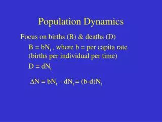
The change in population per time unit can obviously be expressed as the difference between birth rate and death rate. It is reasonable to assume that both the birth rate and the death rate are proportional to the population: and therefore: · P = BR - DR BR = kBR· P DR = kDR· P · (kBR -kDR ) ·t P = (kBR - kDR ) · P P(t) = P0·e Exponential Growth I
Populations of all species grow exponentially over time. This is also true for human beings! Every species eventually outgrows its resources. In the ultimate instance, populations are controlled by hunger, rather than brains. (kBR -kDR ) ·t P(t) = P0·e Exponential Growth II The primary purpose of studying population dynamics is to learn to deal with this depressing law of nature.
As food gets scarce, i.e., as soon as all available food is being consumed by the population, we can determine the food per capita as the total food divided by the population: If not enough food is available, the birth rate will decrease, and the death rate will increase. This is called the crowding effect. The most commonly used assumption is that a one-species ecosystem can support a fixed number of animals of the given species: Fp.c. = Ftotal / P · P P = k · (1.0 - ) · P Pmax Limits to Growth
The above equation is called the continuous-time logistic equation. · Exponential growth Saturation P P = k · (1.0 - ) · P Pmax The Logistic Equation Pmax = 1000
Applying the forward-Euler integration algorithm: to the differential equation describing the population change: we get a difference equation: It may be justified to use this much cruder model, either because the accuracy of our model is not all that great anyway, or because a population may reproduce only in spring (h = 1.0). · P = k · P · P(t+h) = P(t) + h · P(t) Continuous-time vs. Discrete-time Model P(t+h) = P(t) + h · k · P(t) = (1.0 + h·k) · P(t)
The Chain Letter I • Population dynamics modeling techniques may also be applied to macroeconomic modeling. Let us consider the model of a chain letter. • The following rules are set to govern this (artificial) model: • A chain letter is received with two addresses on it, the address of the sender, and the address of the sender’s sender. • After receiving the letter, a recipient sends $1 to the sender’s sender. He or she then sends the letter on to 10 other people, again with two addresses, his (or her) own as the new sender, and the sender’s address as the new sender’s sender. • The letter is only mailed within the U.S. • Every recipient answers the letter exactly once. When a recipient receives the same letter for a second or subsequent time, he (or she) simply throws it away.
The Chain Letter II • Special rules are needed to provide initial conditions. • Every sender has 100 receiver’s receivers, thus is expected to make $100. • Except for the first 11, who don’t pay anything, every sender pays exactly $1. • Hence this is a wonderful (and totally illegal!) way of making money out of thin air. • The originator sends the letter to 10 people without sending money to anyone. • If a recipient receives the letter with only one address (the sender’s address), he or she sends the letter on to 10 other people with two addresses (his or her own as the sender, and that of the originator as the sender’s sender). No money is paid to anyone in this case.
I is the average number of new infections per recipient. R, the number of new recipients, can be computed as the number of new infections per recipient multiplied by the number of recipients one step earlier. R = I · pre(R) P, the number of already infected people, can be computed as the number of people infected previously plus the new recruits. P P = pre(P) + R I = 10 · (1.0 - ) Pmax The Chain Letter III • We can model the chain letter easily as a discrete system.
The Chain Letter IV • We can easily code this model in Modelica.
Simulation Results • Initially, every participant makes exactly $99 as expected. • However, already after seven generations, the entire U.S. population has been infected. • Thereafter, everyone who still participates, loses $1. The energy conservation laws are not violated! No money is being made out of thin air! Those who participate early on, make money at the expense of the many who jump on the band wagon too late.
Exponential growth Stagnation Recession Prosperity Simulation Results
As long as exponential growth prevails, i.e., as long as the second derivative of the population growth is positive, the population is able to borrow money from the future. They effectively eat the bread of their children. Once the inflection point has been passed, the debts made by previous generations have to be paid back. Interpretation
In the U.S., population statistics have been collected once every 10 years since 1850. I used Matlab to fit a logistic model: to the available census data. I then used Modelica to plot the real census data together with the curve fit. · P = a · P + b · P 2 U.S. Census I
Pmax = 402.59 · 106 Inflection point = 1971 We can no longer rely on an increasing number of children to pay for our retirement benefits. U.S. Census III The inflection point is fairly sensitive. Yet, however we compute it, we have already passed it.
Let us look how the curve fitting was done. Since we only have measurement data for the population itself, not for its derivative, we first need to approximate the population gradient. To this end, we lay a quadratic polynomial through three neighboring population data points: Curve Fitting I Pi-1 = c1 + c2· t i-1 + c3· t i-12 Pi = c1 + c2· t i + c3· t i 2 Pi+1 = c1 + c2· t i+1 + c3· t i+12
In a matrix-vector form: } V = Vandermonde matrix c = V -1·p = V \ p Matlab notation Curve Fitting II Pi-1 t i-10 t i-11 t i-12 c1 Pi = t i 0 t i 1 t i 2 · c2 Pi+1 t i+10 t i+11 t i+12 c3 p = V ·c
Now, that we have the coefficient vector, we can approximate the population gradient: Pi = c1 + c2· t i + c3· t i 2 · Pi c2 + 2c3· t i Curve Fitting III • We could equally well have used other interpolation polynomials, such as cubic splines, or inverse Hermite interpolation.
We are now ready to curve-fit the logistic model: We have n equations in the two unknowns a and b. · · · P1 a · P1 + b · P12 P2 a · P2 + b · P22 Pn a · Pn + b · Pn2 · · · We can solve for a and b only in a least-square sense. Curve Fitting IV
In a matrix-vector form: · · · · · · · Pn Pn Pn2 } V = Vandermonde matrix Curve Fitting V · P1 P1 P12 a · · P2 P2 P22 b
In general: x x VT VT VT · · · · y V y V x VT·V · · y Curve Fitting VI
Therefore: VT x (VT·V) -1· VT·y } Penrose-Moore pseudo-inverse x VT·V · · x V \ y y Matlab notation Curve Fitting VII VT·y (VT·V) ·x
When multiple species interact with each other, the simple logistics model no longer suffices. A simple two-species model with one species feeding upon another was proposed by Lotka and Volterra. The Lotka-Volterra model makes the assumption that the predator population without prey would die out by exponential decay, whereas the prey population would grow beyond all bounds due to an unlimited supply of its own food. · Ppred = -a · Ppred + k · b · Ppred · Pprey · Pprey = c· Pprey-b · Ppred · Pprey Predator-Prey Models I
When predator meets prey (Ppred · Pprey ), a certain percentage of the “energy” stored in the prey population is transferred to the predator population. The efficiency of the feeding is less than 100%. Thus, some energy is lost in the process (k < 1.0). Lotka-Volterra models lead to cyclic oscillations, as they are indeed frequently observed in nature. Especially insect populations, such as locust, seem to show up in large numbers in fixed time intervals, whereas they are almost extinct in between. Predator-Prey Models II
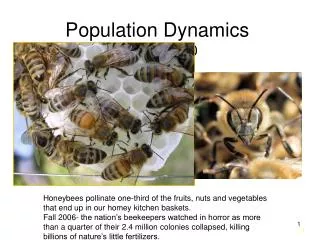
The larch bud moth is an insect that lives in the upper Engiadina Valley of Southeastern Switzerland, at altitudes between 1600 – 2000 m. Its larvae feed on the needles of the larch trees. The population has a cycle time of exactly nine years, i.e., once every nine years, the insect population is larger by several orders of magnitude, and all the larch trees turn brown because of them. Hence the larch bud moth population was curve-fitted to the predator population of a Lotka-Volterra model. The Larch Bud Moth I
The curve fit is excellent indeed. Does this mean that we now understand the population dynamics of the larch bud moth? Unfortunately, the answer to this question is a decided no. The Larch Bud Moth II
The larch bud moth is also plagued by parasites. Thus, if the insect population is large, the chances of spreading the parasites among them grows drastically. Thus, it may make equally much sense to curve-fit the larch bud moth population to the prey population of a Lotka-Volterra model. This was attempted as well. The Larch Bud Moth III
The curve fit is equally excellent. Thus, we cannot conclude from the quality of the curve fit alone that the underlying model represents correctly the cause-effect relationship of the biological system. The Larch Bud Moth IV
Curve fitting can only be used for the purpose of interpolation in space and extrapolation in time (as long as the predicted variables stay within their observed ranges). Models obtained inductively by curve-fitting a mathematical model to a set of observed data should never be used to explain the internal variables of the model. Such a model has no internal validity. A better (internally valid) larch bud moth model shall be presented later. The Dangers of Curve Fitting
Two species can also interact with each other in other ways. They can e.g. compete for the same food source: or they can cooperate, e.g. in a symbiosis: · x1 = a · x1-b · x1 · x2 · x2 = c · x2-d · x1 · x2 · x1 = -a · x1+b · x1 · x2 · x2 = -c · x2+d · x1 · x2 Competition and Cooperation I
Animals of a single species can also cooperate, e.g. by protecting each other in a herd (grouping). or they can suffer from crowding: Of course, several of these phenomena can take effect simultaneously. · · x = -a · x +b · x 2 x = a · x -b · x 2 Competition and Cooperation II
We have looked at single-species ecosystems first. We found that these populations always exhibit exponential growth followed by saturation. This behavior can be modeled using the continuous-time logistic model. We have seen that two-species ecosystems often exhibit oscillatory behavior. This behavior can be modeled using the Lotka-Volterra model. In the next class, we shall look at behavioral patterns exhibited by multi-species ecosystems. Conclusions
Cellier, F.E. (1991), Continuous System Modeling, Springer-Verlag, New York, Chapter 10. Cellier, F.E. (2002), Matlab code to curve-fit a logistic model to the U.S. census data. Cellier, F.E. and A. Fischlin (1982), “Computer-assisted modeling of ill-defined systems,” in: Progress in Cybernetics and Systems Research, Vol. 8, General Systems Methodology, Mathematical Systems Theory, Fuzzy Sets (R. Trappl, G.J. Klir, and F.R. Pichler, eds.), Hemisphere Publishing, pp. 417-429. References