Download
1 / 41
420 likes | 506 Views
Learn about FFT for efficient polynomial multiplication & signal processing. Understand DFT, signal spectrum, complex roots, FFT algorithms, and applications.

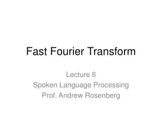
E N D
Polynomial Multiplication with Discrete Fourier TransformFast Fourier Transform FFT
Signal Amplitude or Intensity of, e.g. Voltage Time FFT
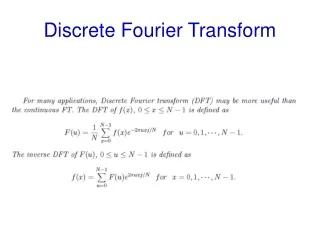
Signal as a linear combination ofsinusoidal waves cos(wt) + i sin(wt) = ei t 2Pi/n, w=2Pi/n, n frequency cycles/time w angular frequency Different components: Strength (and phase) of each component, in frequency domain Add them: aei t u + bei t v + cei t w Signal Spectrum FFT
Digital Signal Amplitude A sequence of numbers, or Time-series FFT
Digital Signal n is same as we considered (order of polynomial) FFT
Signal as a polynomial f(t) = re(i2πωt) ω = a root of equation (xn = 1) n number of roots but all of them are integral powers of w Animation on wiki: http://upload.wikimedia.org/wikipedia/commons/a/a5/ComplexSinInATimeAxe.gif FFT
Omega, or n-th root of 1 Imaginary axis 8 complex roots of x8 = 1 Real axis f(t) = re(i2πωnt) ωn is n-th root, where n is the number of samples on a fixed-length time series
Signals as Functions of roots of 1 Amplitude & Phase f(t) = re(i2πωnt) ωn above, where n is the number of samples FFT
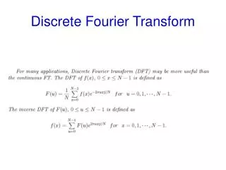
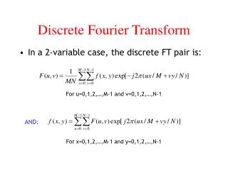
Discrete Fourier Transform (DFT) A sequence of numbers, or Time-series with uniform sampling: (y0, y2, y3, … yn-1) Amplitude Frequency component for f1 = 1/n, n number of samples (= length of time in the unit of sampling interval): (Real_A1, Imaginary_A1) = y0 + y1e(i2Pi/n)*1 + y2e (i2Pi/n)*2 + … A polynomial evaluated on 1st root of 11/n Frequency component for f2 = 2/n: (Real_A2, Imaginary_A2) = y0 + y1ei(1*2Pi/2n)*1 + y2ei(2*2Pi/2n)*2 + … A polynomial evaluated on next root of 11/n …. Frequency component for fn = n/n (one wave over the whole signal length): (Real_A1, Imaginary_A1) = y0 + y1ei(n*2Pi/n)*1+ y2ei(n*2Pi/n)*2 + … A polynomial evaluated on n-th root of 11/n FFT
Discrete Fourier Transform (DFT) Frequency component for f1 = 1/n, n number of samples (= length of time in the unit of sampling interval): (Real_A1, Imaginary_A1) = y0 + y1e(i2Pi/n) + y2e (i2Pi/n)*2 + … A polynomial evaluated on 1st root of 11/n Frequency component for f2 = 2/n: (Real_A2, Imaginary_A2) = y0 + y1ei(2*2Pi/2n) + y2ei(2*2Pi/2n)*2 + … A polynomial evaluated on next root of 11/n …. Frequency component for fn = n/n (one wave over the whole signal length): (Real_A1, Imaginary_A1) = y0 + y1ei(n*2Pi/n) + y2ei(n*2Pi/n)*2 + … A polynomial evaluated on n-th root of 11/n • Polynomial of n-th order: each evaluation takes O(n) time • n evaluations: O(n2) time • Naïve DFT: O(n2) • Recursive Divide and Conquer for evaluating on all simultaneously (FFT): O(n log n) FFT
Signal Processing as Polynomial Multiplication • Not in details: • A digital signal is represented with a polynomial over roots of 1 • “Convolving” is equivalent to Polynomial multiplication FFT
Polynomial Multiplication • f(x) = A0 + A1x1 + A2x2 + . . .+ An-1xn-1 • 2 Representations: • Coefficients (A0, A1, A2, . . ., An-1) • Evaluated at n points y(x0), y(x1), ..., y(xn-1) • Exchangeable: Given A's, evaluate at n points, • or, Given n points, solve for n coefficients • Traditionally: O(n2) algorithms for each. • Divide and Conquer DFT: O(n log n) FFT
Polynomial Multiplication • Given A[0..n-1] DFT evaluates ==> on wn0, wn1, wn2, . . ., wnn-1, • where wn is n-th root of the equation xn = 1 • Takes O(n) for each evaluation, O(n2) for n total points • Recursive divide conquer DFT takes O(n log n) time FFT
Polynomial Multiplication • Given A[0..n-1] DFT evaluates ==> on wn0, wn1, wn2, . . ., wnn-1, • where wn is n-th root of the equation xn -1 = 1 • Takes O(n) for each evaluation, O(n2) for all • Recursive divide conquer DFT takes O(n log n) time • Why evaluate on those complex points, over n roots of 1 (DFT)? • To develop O(n log_n) FFT • for simultaneous evaluation on all of them. • Then convert it to iterative and parallelizable FFT FFT
Primary use of Efficient Polynomial Multiplication Primary use of Efficient Polynomial Multiplication: Convolution of Two Signals Used for filtering Another advantage: wn = e^(i*2pi(theta)/n) = cos(theta) + i*sin(theta), n number of samples This allows us to do Fourier analysis of a signal, e.g. for compression A[] => y() is DFT done by FFT: transforms from time series to its frequency spectrum, and y() => A[] by inverseFFT (or IFFT): transforms a frequency spectrum to time series FFT
Polynomial Multiplication Standard Procedure: A(x) = a0 + a1x1 + a2x2 + … an-1xn-1 B(x) = b0 + b1x1 + b3x2 + … bn-1xn-1 A(x)*B(x) = b0(a0 + a1x1 + a2x2 + … an-1xn-1) + b1x(…) + b2(…) + Example: A(x) = 3 + 2x – 4x2 B(x) = -4 –x + 2x2 A(x)*B(x) = 3*(-4) -x(3+2x- 4x2) +2x2(3+2x-4x2) Total: O(n2) scalar multiplications, where n is order of the two polynomials FFT
Data Structure for Polynomial Coefficient representation (analytical, standard): An = (a0, a1, a2, an-1) Bn = (b0, b1, b3, bn-1) Multiplication: An*Bn = b0(a0, a1, a2, an-1), b1(a0, a1, a2, an-1), …, bn(a0, a1, a2, an-1) Coordinate representation (discrete): Evaluate at n points, (x0, x1, x2, xn-1): An = (x0, y0), (x1, y1), (x2, y2),… (xn-1, yn-1), Each evaluation from : O(n) Total: O(n2) for n points evaluation Why we need n points? FFT
Data Structure for Polynomial Coordinate representation (discrete): Evaluate at n points, (x0, x1, x2, xn-1): An = (x0, y0), (x1, y1), (x2, y2),… (xn-1, yn-1), Each evaluation from : O(n) Total: O(n2) for n points evaluation Why we need n points? To recover each coefficient: n unknowns, with n equations y0 = a0 + a1x0 + a2x02 + … an-1x0n-1 y1 = a0 + a1x1 + a2x12 + … an-1x1n-1…. … yn-1= a0 + a1xn-1 + a2xn-12 + … an-1xn-1n-1 Complexity of this conversion? FFT
Polynomial Multiplication Poly-multiplication in coordinate representation: Evaluate at n points: A(x) = 3 + 2x – 4x2 , B(x) = -4 –x + 2x2 x=(1, 2, 3) A(1) = 1, A(2)=-9, A(3)=-27 B(1) = -1, B(2)=2, B(3)=11 Multiply point by point: R(1)=-1, R(2)=-18, R(3)=-297, R as resulting polynomial Solve for coefficients of R: linear algebra / simultaneous eq solving FFT
Polynomial Multiplication Another way: Evaluate at n points: A(x) = 3 + 2x – 4x2 , B(x) = -4 –x + 2x2 x=(1, 2, 3) A(1) = 1, A(2)=-9, A(3)=-27 B(1) = -1, B(2)=2, B(3)=11 Multiply point by point: R(1)=-1, R(2)=-18, R(3)=-297, R as resulting polynomial Solve for coefficients of R: linear algebra / simultaneous eq solving How many terms? Coefficients? Order of R? Goes up to 4th power of x: r0, r1, r2, r3, r4 Can be handled by increasing power of A and B with 0 coefficients: A(x) = 3 +2x -4x2 +0x3 +0x4 +0x5 , B(x) = … and evaluating at 6 points, not 3: so that we can recover 6 coefficients FFT
Polynomial Multiplication by evaluated points Evaluation at each point: O(n) multiplications at x, x2, x3, … Evaluation at n points: O(n2) Multiplication for n points: O(n) Inverse matrix to solve for coefficients: O(n2) Total poly-mult: O(n2), no advantage over standard way FFT
DFT for Polynomial Multiplication (0) Pad each polynomial to (2n-2)-th order by extending: an=0, an+1=0, ..., a2n-1=0 (1) Evaluate each polynomial at the 2n-th complex roots of 1: w2n0=1, w2n1=wn, w2n2, w2n3, ..., w2n2n-1 (2) Then, element-to-element multiply values at each evaluated pts above: A(wnk)*b(wnk) =: C(wnk), for k=0 … 2n-1 (3) Find coefficients of resulting polynomial C(x) by using w0 through w2n Steps 1 & 3 each takes O(2n log2n), & Step-2 takes O(2n) Total O(n logn) FFT
ωn, n roots of xn=1 ωn =e(i2π/n) ω81 ω80 FFT
ωn, n roots of xn=1 8 roots of x8 = 1 ω81 =e(i2π/8) k-th power: (ω81)k =ek(i2π/8) k-th root: ω8k =ek(i2π/8) ω82 = ω41 ωn =e(i2π/n) n is number of coefficients, in nearest power of 2 ω81 FFT
ωn, n-th root of xn=1 ω82 = ω41 Lower order roots and of higher order roots overlap ω81 So, for A(x) = 3 + 2x – 4x2 +0x3, We will evaluate at four points: ω41= i, ω42= -1, ω43= -i, ω44 =1 FFT
Advantage of using complex roots of one: Divide and Conquer can be faster A(x) = 3 + 2x – 4x2 +0x3 , to be evaluated at 4 points ω1 , ω2 , ω3 , ω4 Modulo nature reduces actual number of computations Specifically, rules (theorems/lemmas) used are: ωnn/2 = ω2 = -1 (second root of x2=1, mid point of roots of any order) ωnn =1 (first root, or 0-th root of any order) (ωnk+n/2)2 = (ωnk)2 (modulo nature) 8 roots of x8 = 1 ω81 =e(i2π/8) k-th power: (ω81)k =ek(i2π/8) k-th root: ω8k =ek(i2π/8) FFT
D&C Polynomial Evaluation A8(x) = a0 + a1x + a2x2 + a3x3 + a4x4 + a5x5 + a6x6 + a7x7 = (a0 + a2x2 + a4x4 + a6x6) + x(a1 + a3x2 + a5x4 + a7x6) = [(a0 + a4x4) + x2(a2 + a6x4)] + x[(a1 + a5x4) + x2(a3 + a7x4)] A polynomial may be written as, A(x) = A0(x2) + xA1(x2) where, A0(z) = a0 + a2z + a4z2 + … + an-2zn/2-1 A1(z) = a1 + a3z + a5z2 + … + an-1zn/2-1 Presuming, n = 2k, the rewriting may recursively go on until k=0. Hence, divide and conquer FFT
D&C Polynomial Evaluation A8(x) = a0 + a1x + a2x2 + a3x3 + a4x4 + a5x5 + a6x6 + a7x7 = (a0 + a2x2 + a4x4 + a6x6) + x(a1 + a3x2 + a5x4 + a7x6) A4(x2) + x A’4(x2) = [(a0 + a4x4) + x2(a2 + a6x4)] + x[(a1 + a5x4) + x2(a3 + a7x4)] A2((x2)2) + (x2)A’2((x2)2) + … Divide and conquer can be now used for evaluating at a value of x. Higher order polynomials from lower order ones, with appropriate coefficients. Now evaluate at all n roots of 1 (DFT): x = ωn0through ωnn-1 Fast Fourier Transformation (FFT) combines these computations using modulo properties of roots of 1 FFT
Discrete Fourier Transformation: D&C Polynomial Evaluation T(n) = 2T(n/2) + n/2 , for the loop (10): O(n) By Master’s theorem: T(n) = O(n log_n) FFT
Polynomial Multiplication by evaluated points There will be 2n point-to-point mult, After the two polynomials are evaluated FFT
Computing the coefficients from points : interpolation DFT: Y = VA Inverse DFT: Solving simultaneous equations Needs inversion of V matrix: Usually, O(n2) operation FFT
Computing the coefficients from points : interpolation • A polynomial evaluation at ωn-1 • Use the same DFT • with ωn-1 • O(n logn) FFT
Computing the coefficients from points : interpolation Solving simultaneous equations to find coefficients vector A: A = V-1Y: but V-1kj = 1/(n* Vjk) Use ωn =e(-i2π/n)in line 4 of DFT, and divide the final returned vector by n FFT
Fast Fourier Transform: FFT FFT: Iterative version of DFT BIT-REVERSE-COPY: shuffle input vector FFT
Evaluate 2 – x + 3x2 +4x3 -2x4 -2x6 +x7 At eight roots of x8=1 2 ω20 =e(i2π/2)*0 =1 -1 3 =1 -4 1 0 -2 1 FFT
3 +1*1 = 3 3 2 ω20 =e(i2π/2)*0 =1 -1 =1 3 11*1 = 2 3 +1*(-2) = 1 3 =1 -4 3 -1*(-2) = 5 1 0 -2 1 FFT
2 1 +i*5 2 -1*1 = 1 -1 3 1 -i*5 =i -4 3 -1*(-2) = 5 1 0 -2 1 e(i2π/4)*1 = cos(Pi/2) + i sin(Pi/2) = i FFT
3 4 2 1 +i*5 1 -1 3-1=2 1 3 1 -i*5 =i 5 -4 -1 1 -1 0 -3 -2 -5 1 e(i2π/8)*1 = cos(Pi/4) + i sin(Pi/4) = (1/sqr-root_2)(1+i) FFT