Download
1 / 24
240 likes | 264 Views
This text explains the concepts of probability and the normal distribution in statistics, with a focus on z-scores and describing correlations. It covers topics such as flipping coins, binomial distribution, and the unit normal table. The text provides clear explanations and examples to help readers grasp these important statistical concepts.

E N D
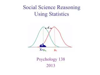
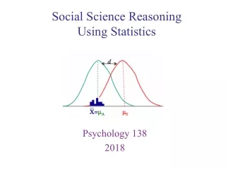
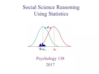
Social Science Reasoning Using Statistics Psychology 138 2017
Exam 2 is Wed. March 8th • Quiz 4 • Fri March 3rd • Covers z-scores, Normal distribution, and describing correlations Announcements
Transformations: z-scores • Normal Distribution • Using Unit Normal Table • Today’s lecture puts lots of stuff together: • Probability • Frequency distribution tables • Histograms • Z-scores Today Start the quincnux machine Outline
Number of heads HHH 3 HHT 2 HTH 2 HTT 1 THH 2 THT 1 TTH 1 TTT 0 Flipping a coin example
.4 .3 probability .2 .1 .125 .375 .375 .125 0 1 2 3 Number of heads Number of heads 3 2 2 1 2 1 1 0 Flipping a coin example
What’s the probability of flipping three heads in a row? .4 .3 probability .2 p = 0.125 .1 .125 .375 .375 .125 Think about the area under the curve as reflecting the proportion/probability of a particular outcome 0 1 2 3 Number of heads Flipping a coin example
What’s the probability of flipping at least two heads in three tosses? .4 .3 probability .2 p = 0.375 + 0.125 = 0.50 .1 .125 .375 .375 .125 0 1 2 3 Number of heads Flipping a coin example
What’s the probability of flipping all heads or all tails in three tosses? .4 .3 probability .2 p = 0.125 + 0.125 = 0.25 .1 .125 .375 .375 .125 0 1 2 3 Number of heads Flipping a coin example
Coin flipping results in The Binomial Distribution As you flip more coins, N = 20 Flipping a coin example
Coin flipping results in The Binomial Distribution As you flip more coins, the binomial distribution can be approximated by the Normal Distribution N = 65 Flipping a coin example
The Normal Distribution (Sometimes called the “Bell Curve”) • Many commonly occurring distributions in nature are approximately Normal Normal Distribution
Defined by density function (area under curve) for variable X given μ & σ2 • Symmetrical & unimodal; Mean = median = mode • ±1 σ are inflection points of curve (change of direction) • The Normal Distribution (Sometimes called the “Bell Curve”) • Many commonly occurring distributions in nature are approximately Normal • Common approximate empirical distribution for deviations around a continually scaled variable (errors of measurement) Galileo Gauss Check out the quincnux machine Normal Distribution
The Normal Distribution (Sometimes called the “Bell Curve”) • Use calculus to find areas under curve (rather than frequency of a score) • We will use a table rather to find the probabilities rather than do the calculus. Normal Distribution
The Normal Distribution (Sometimes called the “Bell Curve”) • Important landmarks in the distribution (and the areas under the curve) • %(μ to 1σ) = 34.13 • p(μ < X < 1σ) + p(μ > X > -1σ) ≈ .68 • %(1σ to 2σ) = 13.59 • p(1σ < X < 2σ) + p(-1σ > X > -2σ) = 27%, cumulative = .95 • %(2σ to ∞) = 2.28 • p(X > 2σ) + p(X < -2σ) ≈ 5%, cumulative = 1.00 100% 95% 68% • We will use the unit normal table rather to find other probabilities 34.13 2.28 13.59 Normal Distribution
Lots of places to get the Unit Normal Table information • But be aware that there are many ways to organize the table, it is important to understand the table that you use • Unit normal table in your reading packet • And online: http://psychology.illinoisstate.edu/jccutti/psych138/resources copy/TABLES.HTMl - ztable • “Area Under Normal Curve” Excel tool (created by Dr. Joel Schneider) • Bell Curve iPhone app • Do a search on “Normal Table” in Google. Resources and tools
.4 .3 probability .2 • We will use the unit normal table rather to find other probabilities .1 .125 0 1 2 3 .875 Number of heads Unit Normal Table
Proportions beyondz-scores • Same p-values for+ and - z-scores • p-values = 0.50 to 0.0013 zp .1359+.0228 = .1587 For z = 1.00 , 15.87% beyond, p(z > 1.00) = 0.1587 1.01, 15.62% beyond, p(z > 1.00) = 0.1562 Note. : indicates skipped rows Unit Normal Table (in reading packet and online)
Proportions beyondz-scores • Same p-values for+ and - z-scores • p-values = 0.50 to 0.0013 For z = -1.00 , 15.87% beyond, p(z < -1.00) = 0.1587 100% - 15.87% = 84.13% = 0.8413 Note. : indicates skipped rows Unit Normal Table (in reading packet)
Proportions beyondz-scores • Same p-values for+ and - z-scores • p-values = 0.50 to 0.0013 For z = 2.00, 2.28% beyond, p(z > 2.00) = 0.0228 2.01, 2.22% beyond, p(z > 2.01) = 0.0222 As z increases, p decreases Note. : indicates skipped rows Unit Normal Table (in reading packet)
Proportions beyondz-scores • Same p-values for+ and - z-scores • p-values = 0.50 to 0.0013 For z = -2.00, 2.28% beyond, p(z < -2.00) = 0.0228 Note. : indicates skipped rows Unit Normal Table (in reading packet)
Proportions left of z-scores: cumulative • Requires table twice as long • p-values 0.0003 to 0.9997 50% + 34.13 = 84.13% to the left Cumulative % of population starting with the lowest value For z = +1, Unit Normal Tablecumulative version (in some other books)
Example 1 Suppose you got 630 on SAT. What % who take SAT get your score or better? 9.68% above this score • Population parameters of SAT: μ = 500, σ = 100, normally distributed From table: z(1.3) =.0968 • Solve for z-value of 630. • Find proportion of normal distribution above that value. Hint: I strongly suggest that you sketch the problem to check your answer against SAT examples
Example 2 Suppose you got 630 on SAT. What % who take SAT get your score or worse? 100% - 9.68% = 90.32% below score (percentile) • Population parameters of SAT: μ = 500, σ = 100, normally distributed From table: z(1.3) =.0968 • Solve for z-value of 630. • Find proportion of normal distribution below that value. SAT examples
Check the quincnux machine • In lab • Using the normal distribution • Questions? • Brandon Foltz: Understanding z-scores (~22 mins) • StatisticsFun (~4 mins) • Chris Thomas. How to use a z-table (~7 mins) • Dr. Grande. Z-scores in SPSS (~7 mins) Wrap up