New quantum lower bound method, with applications to direct product theorems
530 likes | 766 Views
New quantum lower bound method, with applications to direct product theorems. Andris Ambainis, U. Waterloo Robert Spalek, CWI, Amsterdam Ronald de Wolf, CWI, Amsterdam. Query model. i. i. Input x 1 , …, x N accessed by queries. Complexity = the number of queries. 0. 1. 0. 0. x i.

New quantum lower bound method, with applications to direct product theorems
E N D
Presentation Transcript
New quantum lower bound method, with applications to direct product theorems Andris Ambainis, U. Waterloo Robert Spalek, CWI, Amsterdam Ronald de Wolf, CWI, Amsterdam
Query model i i • Input x1, …, xN accessed by queries. • Complexity = the number of queries. ... 0 1 0 0 xi 0 x1 x2 x3 xN
Grover's search ... 0 1 0 0 • Is there i such that xi=1? • Queries: ask i, get xi. • Classically, N queries required. • Quantum: O(N) queries [Grover, 1996]. • Speeds up any search problem. x1 x2 x3 xN
Quantum counting [Boyer et al., 1998] ... 0 1 0 0 • Is the fraction of i:xi=1 more than ½+ or less than ½- ? • Classical: queries. • Quantum: queries. x1 x2 x3 xN
Element distinctness ... 1 3 17 5 • Are there i, j such that ij but xi=xj? • Classically: N queries. • Quantum: O(N2/3). x1 x2 x3 xN
Lower bounds • Search requires N) queries [Bennett et al., 1997]. • Counting: 1/) [Nayak, Wu, 1999]. • Element distinctness: (N2/3) [Shi, 2002].
Lower bound methods • Adversary: analyze algorithm, prove it is incorrect on some input. • Polynomials: describe algorithm by low degree polynomial.
Limits of adversary method • Certificate for f on input (x1, x2, …, xN): set of variables xi which determine f(x1, x2, …, xN). • Search: is there i:xi=1? ... 0 1 0 0 x1 x2 x3 xN
Limits of adversary method • Certificate for f on input (x1, x2, …, xN): set of variables xi which determine f(x1, x2, …, xN). • Search: is there i:xi=1? ... 0 0 0 0 x1 x2 x3 xN
Certificate complexity • Cx(f): the size of the smallest certificate for f on the input x. • Search: C0=N, C1=1.
Limits of adversary method Theorem [Spalek, Szegedy, 2004] • Any quantum adversary lower bound is at most
Example:element distinctness ... 1 3 17 5 • Are there i, j:xi= xj? • 1-certificate: {i, j}, xi= xj. • Adversary bound: • Actual complexity: O(N2/3). x1 x2 x3 xN
Example: triangle finding • Graph G, specified by N2 variables xij: xij=1, if there is edge between i and j. • Does G contain a triangle? • 1-certificate:{ij, jk, ik}, xij= xik= xjk=1. • Adversary lower bound: at most • The best algorithm: O(N1.3) [MSS 03].
Quantum query model • Fixed starting state. • U0, U1, …, UT – independent of x1, x2, …, xN. • Q – queries. • Measuring final state gives the result. U0 Q Q U1 … UT
Queries • Basis states for algorithm’s workspace: |i, z, i{1, 2, …, N}. • Query transformation: • Example: • |i, z|i, z, if xi=0; • |i, z-|i, z, if xi=1;
| • Two registers: HA, HI. • Query Q: Adversary framework Quantum algorithm A x1 x2 … xN
Example:Grover search • Start state: |start|0, • End state
Density matrices • Measure HA, look at density matrix of HI
Density matrices • Sum of off-diagonal entries. • N(N-1) entries. • Sum for starting state: • Sum for end state: 0. • Query changes the sym by at most 2N. • (N) queries needed.
Limits of this approach • (end)x, y measures the possibility of distinguishing x from y. • If every (end)x, y small, we can, given x, y: f(x)f(y), distinguish x from y.
Limits of this approach • It might be that: • Every x can be distinguished from every y; • There is no measurement that distinguishes all x from all y. Adversary method fails quantum algorithm f(x)=0 f(y)=1
K-fold search ... 0 1 0 0 • K items i:xi=1, find all of them. • O(NK) queries: O(N/K) for each item. • This is optimal. x1 x2 x3 xN
Direct product theorem • Theorem [KSW 04] Solving K-fold search with success probability c-K, c>1 requires NK queries. • Easy to prove for success probability c. • Difficult for probability c-K. Why is this useful????
Application:sorting • Theorem [KSW04] A quantum algorithm for sorting x1, x2, …, xN with S qubits of workspace must use queries.
Proof • Divide algorithm into stages: first K items sorted, next K items sorted, … • Suffices to show each stage requires (NK) queries. • Each stage reduces to K-fold search.
Proof • At the beginning of ith stage, we get S qubits from the previous stage. • Theorem K-fold search requires (NK) queries, even if we allow K/C qubits of advice.
Proof • Theorem K-fold search requires (NK) queries, even if we allow K/C qubits of advice. • Proof Replace advice by completely mixed state. • Success probability p with advice => Success probability p2-K/C, no advice.
Direct product theorem • Theorem Solving K-fold search with success probability c-K, c>1 requires NK queries. • [KSW 04]: proof by polynomials method. • This talk: (new) adversary method.
Proof sketch • “Know-0”, “Know-1”, …, “Know-k” states. • Describe quantum state as
Proof • Adversary framework • Start state for input: Quantum algorithm A | x1 x2 … xN
Proof • State of HI if we know • Subspace Tj spanned by all
Proof • T0T1… TK. • T0 – starting state. • TK – entire HI. T0 T1 …. TK Tj – “know at-most j” subspace
Proof • Sj=Tj(Tj-1). T0 T1 … TK
Proof • Sj=Tj(Tj-1). T0 S1 … SK Sj is “know-j” subspace.
Proof • | - state of algorithm including the input register |x1 … xN. |j belongs to HA Sj. • Probability of “know-j”:
Proof • Start state: p0=1, p1=…=pK=0. • Change in one query: • After NK queries, pK/2+1, …, pK are exponentially small. • Success probability exponentially small.
Threshold functions ... 0 1 0 0 • F(x1, x2, …, xN)=1 if xi=1 for at least t values i{1, 2, …, N}. • F(x1, x2, …, xN)=0 if xi=1 for at most t-1 values i{1, 2, …, N}. • Query complexity: (Nt). x1 x2 x3 xN
Threshold functions ... 0 1 0 0 • F(x1, x2, …, xN)=1 if xi=1 for at least t values i{1, 2, …, N}. • F(x1, x2, …, xN)=0 if xi=1 for at most t-1 values i{1, 2, …, N}. • Query complexity: (Nt). x1 x2 x3 xN
Threshold functions • K instances of threshold function. • (KNt) queries. • Theorem Solving all K instances with probability at most c-K requires KNt queries.
Proof • K input registers. • Each input register initially , |0, |1 - uniform over |x1 … xN with t-1 and t values i:xi=1. … Algorithm
Proof • For each instance, states “solved”, “know-0”, “know-1”, … “know-(t-1)”. • For K instances, vector of K states. • Progress of a state: • “solved” – progress t/2. • “know-t/2”, … “know-(t-1)” – progress t/2. • “know-j”, j<t/2 – progress j.
Proof • If progress of final state less than tK/4, the probability of getting all K correct answers is c-K. • Decompose current state • Potential function
Proof • Start state: P()=1. • For pj, jtK/4 to be more than c-K, • One query increases P() by at most a factor of
Proof • F(x1, x2, …, xN)=0, “know-j”: • F(x1, x2, …, xN)=1, “know-j”:
Proof • Starting state: • “Solved”: • “Know-j”
Application: testing linear inequalities • aij known, xi, bj accessed by queries. • Which inequalities are true?
Our result • Memory limited to S (qu)bits. • Classically: (N2/S) queries. • Quantum: (N3/2t1/2/S1/2) queries. • Lower bound follows from threshold function lower bound.