Motion Correction in fMRI time series
830 likes | 1.03k Views
Motion Correction in fMRI time series. J.-F. Mangin, L. Freire, A. Roche, C Poupon. Service Hospitalier Frédéric Joliot, CEA, Orsay, France Instituto de Biofisica e Engenharia Biomedica, FCUL, Lisboa, Portugal Instituto de Medicina Nuclear, FML, Lisboa, Portugal

Motion Correction in fMRI time series
E N D
Presentation Transcript
Motion Correction in fMRI time series J.-F. Mangin, L. Freire, A. Roche, C Poupon Service Hospitalier Frédéric Joliot, CEA, Orsay, France Instituto de Biofisica e Engenharia Biomedica, FCUL, Lisboa, Portugal Instituto de Medicina Nuclear, FML, Lisboa, Portugal Projet Epidaure, INRIA, Sophia-Antipolis, France Medical Vision Laboratory, Oxford, UK
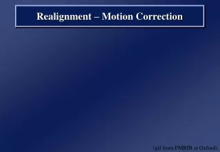
Motion correction, why? Task- correlated motion voxel time series f MRI time series
Some constraints in the scanner to minimize motion Tracking (anatomical or artificial landmarks) On line corrections (MR Echo Navigator) Postprocessing: image registration Which solutions?
Definition: given two images, find the geometrical transformation that « best » aligns homologous voxels Image registration First 3D image Second 3D image
Classification of registration problems • Search space (rigid, non-rigid) • Monomodal / multimodal • Intra-subject / inter-subjects
Given two images I et J, Optimization scheme Similarity measure Search space (rigid, affine, spline, etc.) General formulation of image registration
Geometric Approach Detect features (points, lines, surfaces,… graphs) Measure the distance between these features Building a similarity measure • Iconic Approach • Direct comparison of intensities
How to register these images ? Intuitive example
Measure: for instance, Geometric/IconicApproach Feature detection (here, points with high curvature)
Measure: for instance, Geometric/Iconic Approach Feature detection (here, points with high curvature)
Measure: e.g., Interpolation: T Geometric/Iconic Approach No segmentation!
T1 =Id Geometric/Iconic Approach The simple case of binary images… No segmentation! Measure: e.g.,
Partial overlap T2 Geometric/Iconic Approach No segmentation! Measure: e.g.,
Iconic approach for fMRI! A lot of widely used softwares: SPM, AIR, AFNI, etc. Minimize the sum of squared differences Search through rigid motions (sometimes affine) A typical fMRI image of the nineties
Fighting with local optima Improving accuracy Main differences between softwares? • Preprocessing (smoothing) • Interpolation • Optimization scheme (iterative) spline nearest neighbor linear • Powell • Levenberg Marquardt • Modified Gauss-Newton
Iterative optimization of smooth measure Small motion = good initialization
Is everything fine? Block design, 3T magnet 18 frames (2 sec/frame) Activations? versus 180 frames t Motion correction
Motion-related artifacts: intrascan motion; the spin history effect; interaction between motion and susceptibility; Non perfect estimation and interpolation. The consequences of motions Task-correlated motion = Confounds in cognitive analysis Use motion estimations as regressors?
BUT! Could activated areas be responsible For the task-correlated motion estimation? Is this monomodal situation so secure?
Intensities of image I Intensies of image J Classification of standard similarity measures • Assumed relationship: Conservation of intensity • Adapted measures : Sum of squared differences Sum of absolute differences
Correlation coefficient Classification of standard similarity measures • Assumed relationship: Affine Intensities of image I • Adapted measures Intensies of image J Ratio of image uniformity (Woods)
Classification of standard similarity measures • Assumed relationship: Intensities of image I Functional • Adapted measures Intensies of image J Woods criterion (1993) Woods variants (Ardekani, 95; Alpert, 96; Nikou, 97) Correlation Ratio (Roche, 98)
Classification of standard similarity measures • Assumed relationship: Statistical Intensities of image I • Adapted measures Intensies of image J Joint entropy (Hill, 95; Collignon, 95) Mutual Information (Collignon, 95; Viola, 95) Normalized Mutual Information (Studholme, 98)
Do activated areas bias Least Square approaches? LS-SPM (Friston); LS-AIR (Woods); GM - custom (INRIAlign); RIU-AIR (Woods); CR – custom (Roche) MI - custom (Wells, Maes, Viola). Confounds related to interpolation method or search method ? In some experiments LS - Custom; RIU - Custom; IPMI’01 II. Methods Similarity Measures Let us compare various methods… The “sum of squared differences” measure assumes Gaussian noise for the difference between both images…
Define a joint probability distribution: Generate a 2-D histogram where each axis is the number of possible greyscale values in each image Each histogram cell is incremented each time a pair (I_1(x,y), I_2(x,y)) occurs in the pair of images If the images are perfectly aligned then the histogram is highly focused. As the images mis-align the dispersion grows recall Entropy is a measure of histogram dispersion Entropy for Image Registration
Define joint entropy to be: Images are registered when one is transformed relative to the other to minimize the joint entropy The dispersion in the joint histogram is thus minimized Using joint entropy for Image Registration
Commonly used definitions: I(A,B) = H(A) + H(B) - H(A,B) Maximizing the mutual info is equivalent to minimizing the joint entropy (last term) This definition is related to the Kullback-Leibler distance between two distributions Definitions of Mutual Information
Aim of the comparison of methods: assess the potential bias in motion parameter estimation due to activation presence, whatever the actual accuracy of each method. Accuracy study has been done in several works (Jiang, Frouin, West, Holden, etc.), and requires the study and optimization of each parameter influence, which is far beyond the scope of this work. This is not a robustness or accuracy study ! IPMI’01
Brucker scanner operating at 3T using a 30 contiguous slice 2D EPI sequence (slice array of 64x64 voxels). Pixel size of 3.75mm and slice thickness of 4mm. Various simulated time series. Actual time series using a block design. A few words about the datasets IPMI’01 II. Methods Image Acquisition
Simulated Activation Patterns IPMI’01 A first pattern inferred from a simple visual experiment Two smaller patterns stemming from erosion of the initial largest pattern Pattern A1 A2 A3 Size (%) 12.4 6.2 3.2 Mean(%) 1.26 1.19 1.18 Max(%) 2.04 2.03 2.03
Design of Simulated Time Series IPMI’01 3x3x3 median filtering Tsim applied. 62x62x28 geometry. Gaussian/Rician noise (=2.5%) Activation pattern Reference image Test images n 1 2
I Simulated Activations Without Motion + x 0 1 2 39 40 3-D Frames Test,1 Test,2 Test,39 Run the six registration methods and evaluate thetransformation parameters (tx, ty, tz, rx, ry, rz) for each package. Compute cross-correlation between each parameter and A1 time course and infer activated areas.
I A couple of estimated motion parameters
I Detection of “activated areas” using General Linear Model Spatial Gaussian smoothing - 5mm Low-pass filtering with 2-frame width Voxels activated if p-value > 0.001 Spurious Clustered Voxels (false positives) LS-SPM – 227 LS-AIR –16 RIU-AIR and MI - 0
Simulated activations with simulated motion II IPMI’01 1 2 20 t=0.1mm 1 2 20 Tsim t=5.0mm r=0.1deg 1 2 20 r=2.0deg t = 0.1, 0.2, 0.5, 1.0, 2.0 and 5.0 mm r = 0.1, 0.2, 0.5, 1.0, and 2.0 deg
8 Different Reference Images Nº Pattern Mean Signal Increase (%) 1 NA NA 2 A1 0.63 3 A1 1.26 4 A1 2.52 5 A1 5.04 6 A1 10.08 7 A2 2.52 8 A3 2.52 Simulated activations with simulated motion II
Simulated activations with simulated motion IIA IPMI’01 Influence of motion amplitude - 2 Reference images: Pattern Mean Signal Increase (%) 1 NA NA 2 A1 0.63 3 A1 1.26 4 A1 2.52 5 A1 5.04 6 A1 10.08 7 A2 2.52 8 A3 2.52 - Test images: t = 0.1, 0.2, 0.5, 1.0, 2.0, 5.0 mm. r = 0.1, 0.2, 0.5, 1.0, 2.0 deg.
Simulated activations with simulated motion IIB IPMI’01 Influence of activation amplitude - 6 Reference images: Pattern Mean Signal Increase (%) 1 NA NA 2 A1 0.63 3 A1 1.26 4 A1 2.52 5 A1 5.04 6 A1 10.08 7 A2 2.52 8 A3 2.52 - Test images: t = 0.2 mm. r = 0.2 deg.
Simulated activations with simulated motion IIC IPMI’01 Influence of activation size - 4 Reference images: Pattern Mean Signal Increase (%) 1 NA NA 2 A1 0.63 3 A1 1.26 4 A1 2.52 5 A1 5.04 6 A1 10.08 7 A2 2.52 8 A3 2.52 - Test images: t = 0.2 mm. r = 0.2 deg.
We have also performed an additional experiment on the influence of the initial spatial smoothing applied by SPM and AIR RIU-AIR problems are overcome by a large smoothing, but motion estimates turn out to be biased. For SPM, low smoothing implies smaller bias but motion estimates are less accurate. Evaluation of spatial filtering pre-processing effect III IPMI’01
Experiment With Actual Time Series IV IPMI’01 18 frames (2 sec/frame) 180 frames t
Experiment With Actual Time Series IV Statistical Inference: Gaussian smoothing (FWHM 5mm); High-pass temporal filtering (period 120s); Low-pass temporal filtering by a Gaussian function (4s). Two explanatory variables: Periodic stimulus convolved with a standard hemodynamic response; Time derivative of hemodynamic response. Voxels reported activated if the p-value > 0.05.