Download
1 / 39
400 likes | 518 Views
This study explores the significance of sea ice salinity in oceanic models, particularly regarding ice mass balance and circulation. It addresses crucial questions about how sea ice desalination impacts large-scale dynamics and ecosystem modeling. Employing both 1D and 3D modelling techniques, we analyze temperature effects, brine drainage, and salt fluxes under various conditions. Our findings suggest that accurate representation of salinity is vital for predicting changes in Arctic and Antarctic ecosystems. The integration of salinity dynamics is crucial for future climate predictions.

E N D
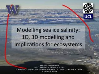
Modelling sea ice salinity: 1D, 3D modelling and implications for ecosystems Martin Vancoppenollecoll.: T. Fichefet, H. Goosse, C.M. Bitz, S. Bouillon, G. Madec, M.A. Morales Maqueda, J.-L. Tison, C. Lancelot, B. Delille, F. Jardon, F. Vivier
Approach and questions • What aspects of sea ice desalination are relevant for large-scale sea ice mass balance and ocean circulation? • How to represent ice salinity in models ? • What are the implications for ecosystem models ?
Why modelling ice salinity ? Variable salinity – S=5 Variable salinity – MY profile Albedo + 10% Simulated change in Arctic sea ice thickness (1979-2006) Vancoppenolle et al., Ocean Modelling, 2009b
Thermal properties of sea ice Thermal properties Diffusion of heat Growth / melt rates
growth / melt drainage Ice-ocean salt / freshwater exchanges Virtual salt flux (upper ocean salinity tendency) Freshwater flux / Salt flux Flushing Snow ice Lateral meltwater flow Congelation Brine drainage Brine drainage Melt Melting ice Growing ice
Outline • 1D modelling • 3D modelling • Perspectives for ecosystems
Is Thermal Effect Important ? h (m) S (ppt) • Sea ice model with brine thermodynamic effect (Bitz and Lipscomb, 1999) • Run for 50 years using climatological forcing • Using with various salinity profiles Vancoppenolle, Fichefet and Bitz (GRL 2005)
How we model ice salinity (1D) ? • Thermal equilibrium • All salt is locked within brine inclusions • Salt transport breaks equilibrium • m = freezing point salinity-temperature ratio [0.054 °C/ppt] • e = brine volume frac. [-] • S = ice bulk salinity [ppt] • T = ice temperature [°C] • s = brine salinty [ppt] • vz = percolation velocity (function of meltwater production) [m/s] • Ds = salt diffusivity in brine [m2/s]
Parameterizing Brine Drainage Gravity Drainage • Convection if Ra is >5 (Notz & Worster, 2008) Flushing • Percolation if • Surface melting • min(e) > 5% • 30 % of meltwater percolates (Vancoppenolle, Bitz and Fichefet, JGR 2007) Vancoppenolle, Goosse, et al. (JGR 2010)
1d Simulations of Brine Drainage Summer desalination of Arctic sea ice(Vancoppenolle, Bitz and Fichefet, JGR 07) Multiyear desalination of Arctic sea ice (Vancoppenolle, Fichefet and Bitz, JGR 06) Desalination of Antarctic sea ice (Vancoppenolle, Goosse et al., JGR 10)
Winter desalination is sensitive to diffusivity parameterization Turbulent diff. Model (solid) Obs (dash) Molecular Diff. Winter salinity profileData from Tison et al.
Winter desalination is sensitive to diffusivity parameterization Antarctic sea ice simulations, June.
Summer desalination is sensitive to model parameters Brine volume fractionpermeability threshold Penetration of penetrating radiation Fraction of vertical percolation 10% 0.2 0 8% 0.3 0.3 5% 0.5 0.5 Simulated surface salinity at Point Barrow (Alaska), June, for several sensitivity exps.
Sensitivity to parameters and forcing: summary • Gravity drainage • Diffusivity parameters • Critical rayleigh number • Turbulent diffusivity • Flushing • Snow depth • Superimposed ice formation • Penetration of radiation (io) in the ice • Fraction of meltwater that is allowed to percolate vertically • Brine volume fraction permeability threshold
Full-depth convection 1 – 2 – 3 – 4 1 – 2 – 4 – 3 4 – 3 – 2 - 1 4 – 3 – 2 – 1 Results of a run in Antarctic sea ice with high snowfall Sep 17 (1 – thin solid); Sep 24 (2 – dot); Oct 1 (3 – solid thin); Oct 8 (dash)
Approach • Problems: • Ice thickness categories • Advection of tracers is expensive • Approach: develop a simple S equation • 1 equation for vertical mean salinity • Shape of profile function of vertical mean salinity • Include this simple S equation LIM • Salt content (S.h) for each ice category • Horizontal transport (Prather, 86) • Remapping in thickness space (Lipscomb, JGR01) • Ridging / Rafting Red diam: OBSSolid: Simple eq. Dash: Transport eq. Comparison at Point Barrow (AK) Vancoppenolle et al. (OM 2009a, 2009b)
Simulated Hemispheric Mean Salinitywith a 3D Ice-Ocean ModelForced by Reanalyses Hemispheric mean ice salinity simulated by NEMO-LIM3:Arctic (black) and Antarctic (grey). (différences hémisphériques : percolation, glace blanche, âge de la glace + cycle saisonnier, variablité interannuelle)
Mar Jun Sep Dec S (‰) hi(m) Icesalinity vs thickness in the model and fromCox and Weeks (1974) regressionscomputedusingicecore data Comparison to Obs Comparison to observations in variousregions(compilation from > 1000 cores)
Sep Mar Mar Sep. Geographical Distribution • Arctic • Winter maximum • In winter, salinityreflectsthickness / age of seaice • Summer low / constant values • Antarctic • Weakearcontrasts • Fall maximum • Local maxima due to polynyas and maximum snowfall Ice salinity (1979-2006) averaged overice thickness categories
Impact (Arctic) 2 configurations Prescribed salinity Simulated salinity Ice thicker for varying salinity Differences up to 1m Difference in volume ~ 10% More ice growth at the ice base (due to reduced energy of melting) More surface melt(due to reduced specific heat) More bottom melt(enhanced ice-albedo feedback) Varying – prescribed salinity 1979-2008 Annual mean thickness difference Vancoppenolle et al., 2009b
Impact (Antarctic) Varying – prescribed salinity Mean 1979-2009 Ice thickness difference • 2 configurations • Prescribed salinity • Simulated salinity • Ice thicker for varying salinity • Mean volume difference ~ 20% • Importance of ice-ocean interactions • Including variations of S • Induce more ice formation with less salt rejection • Reduces vertical mixing in the upper ocean • Reduces the oceanic heat flux • Increases sea ice formation Vancoppenolle et al., 2009b
Impact on Upper Ocean Mean 1979-2006 difference in sea surface salinity Varying - prescribed Varying – prescribed S
Why modelling salinity ?2) Ecosystems • Biophysical couplings associated with ice salinity • Nutrient distribution • Diatom transport mode • Brine salinity inhibition of growth • Brine volume fraction Vertical structure of ice ecosystems
Modelling Sea Ice Ecosystems • Energy-conserving thermodynamics and salt transport • 1-stream Beer law with attenuation by chlorophyll-a • Tracer transport • Ecosystem model (diatoms and silicates)
Brine-Ecosystem Coupling • Ecosystem variables (n=1, 2) (diatoms=DAF, silicates=DSi) • C = bulk concentration • z = brine concentration • e = brine volume fraction • Evolution equation • Physical sources & sinks
Comparison to Observations After calibration of µ, l, ws December Chlorophyll-a profile solid black: simulated (dots = STD) horizontal lines: obs at ISPOLred : double snow
Role of diatom transport mode • Different scenarios: • (a) diatoms follow brine motion • (b) diatoms are locked in ice without following brine motion • (c) diatoms follow brine motion and stick on brine inclusion walls • Observations • Highest biomass is achieved if algae move with brine and stick on brine’s walls. • If algae are not sticky but mobile, they are rejected of the ice as salt, which inhibits the community development. • The nutrient pump increases the availability of nutrients and hence promotes community development. Total biomass (mg chl-a/m2) as a function of time (months) for the different scenarios of brine-biology interactions. Note the log scale on the y axis.
Role of convection on biomass Biomass in silica units Dissolved Silica Total Silica
Why nutrients are not limiting in winter? • Salt is rejected from ice • due to thermodynamic constrains on brine salinity • Common sense: nutrients should be rejected from the ice • Nutrient fluxes are proportional to: • Ocean-brine gradient of nutrient concentration • Diffusivity (high for growing ice) • Hence, nutrients can be fluxed to the ice.time scales of nutrient uptake is much slower than convection
Conclusions (1) • Ice salinity can reasonably well be simulated • 1d models: winter convection, full-depth convection, flushing • Timing, magnitude and model sensitivity are uncertain • Ice salinity is an important actor of large-scale ice-ocean dynamics • Ice salinity affect thermodynamics in the Arctic and ice-ocean interactions in the Antarctic • Ice salinity is increasing now as the amount of FY ice increases. Hence, the sensitivity of coupled models may depend on how salinity could be represented
Conclusions (2) • Brine-ecosystem multi-layer models are quite different from single-layer based models • Brine dynamics allow to simulate vertical structure in ecosystem in a reasonable way • There are brine dynamics-nutrient interactions • Transport mode of diatoms is important • Brine salinity limitation is the second important factor after light limiation
Remaining problems (1) • No thermo-haline coupled term in brine transport equations • Physical inconsistencies in the model (ice/brine density, freezing point, …) • Model results rely on uncertain parameterizations
Remaining problems (2) • Non-destructive method-based time series • Better account of spatial variability (Hajo’s talk) • Less errors at high brine volumes (Phillip’s talk) • How should vertical diffusivity be parameterized ? • Permeability-porosity relation for wide range of T,S • What are the pathways of seawater during surface flooding ? • Full-depth convection: when, how, how often ? • How to represent 3D subfloe-scale circulations ? • What is the impact of ridged ice desalination? • How to represent gas transfer? • How to design a sound model-data comparison
The truth about Louvain-la-Neuve Ice Model nice model huh? I found inspiration from an African instrument, but I improved it… The principle is very basic: A terrific vibration with maximal resonance… THANKS TO: Cc Bitz, Ralph Timmermann, Steve Ackley, Thierry Fichefet, HuguesGoosse, GurvanMadec and NEMO team, Jean-Louis Tison, Tony Worby, HajoEicken, Bruno Delille, Miguel Angel Morales Maqueda, Bruno Tremblay, IouliaNikolskaia , OiivierLecomte, Olivier Lietaer, Sylvain Bouillon, Anne de Montety, Christiane Lancelot and Ivan Grozny + forgotten!
Further reading • Vancoppenolle, M., H. Goosse, A. de Montety, T. Fichefet, B. Tremblay and J.-L. Tison (2010). Modelling brine and nutrient dynamics in Antarctic sea ice : the case of dissolved silica. Journal of Geophysical Research, 115(C2), C02005, doi:/10.1029.2009JC005369. • Vancoppenolle, M., T. Fichefet, H. Goosse, S. Bouillon, G. Madec and M.A. Morales Maqueda (2009a). Simulating the mass balance and salinity of Arctic and Antarctic sea ice. 1. Model description and validation, Ocean Modelling, 27, 33-53, doi:10.1016/j.ocemod.2008.10.005. • Vancoppenolle, M., T. Fichefet, and H. Goosse (2009b). Simulating the mass balance and salinity of Arctic and Antarctic sea ice. 2. Importance of sea ice salinity variations, Ocean Modelling, 27, 54-69. • Vancoppenolle, M. (2008b). Modelling the mass balance and salinity of Arctic and Antarctic sea ice, Phd Thesis, Université Catholique de Louvain, ISBN 978-2-87463-113-9. • Vancoppenolle, M., C. M. Bitz, and T. Fichefet (2007), Summer landfast sea ice desalination at Point Barrow, Alaska: Modeling and observations, Journal of Geophysical Research, 112, C04022, doi:10.1029/2006JC003493. • Vancoppenolle, M., T. Fichefet and C.-M. Bitz (2006) : Modeling the salinity profile of undeformed Arctic sea ice, Geophysical Research Letters, L21501, doi://2006GL028342. • Vancoppenolle, M., T. Fichefet, and C.M. Bitz (2005) : On the sensitivity of undeformed Arctic sea ice to its vertical salinity profile, Geophysical Research Letters, L16502, doi://2005GL023427.