Investigating the Impact of FDI on Economic Growth in India: A Simultaneous Equation Approach
This study examines the critical role of Foreign Direct Investment (FDI) in promoting economic growth in India over the period from 1999-2000 to 2011-2012. Utilizing simultaneous equation models, we explore the bidirectional relationship between FDI and economic growth, whereby incoming FDI boosts economic growth, and vice versa. The model incorporates variables such as Gross Fixed Capital Formation (GCFC), exports, and labor growth, utilizing methods like 2SLS and 3SLS for estimation, ensuring a robust analysis of the economic dynamics at play.

Investigating the Impact of FDI on Economic Growth in India: A Simultaneous Equation Approach
E N D
Presentation Transcript
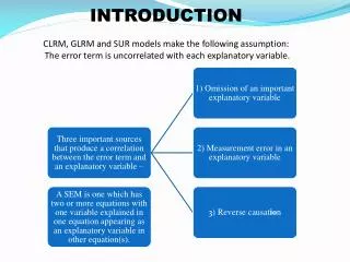
INTRODUCTIONCLRM, GLRM and SUR models make the following assumption: The error term is uncorrelated with each explanatory variable.
Purpose Why SES? • To investigate the importance of FDI for economic growth in India • Time period: 1999-00 to 2011-12 • Bi – directional connection between FDI and economic growth • Incoming FDI stimulates economic growth and in its turn a higher GDP attracts FDI
Model • Growth = a1 + a2*(GCFC) + a3*(FDI) + a4*Export + a5*Labor • FDI = b1 + b2*Growth + b3*GCFC + b4*(Wage) • GCFC = c1 + c2*FDI + c3*Growth + c4*M3 • Export = d1 + d2*Growth + d3*EXRATE + c4*GCFC Reference: FDI and Economic Growth - Evidence from Simultaneous Equation Models, G Ruxanda, A Muraru - Romanian Journal of Economic Forecasting, 2010. http://www.ipe.ro/rjef/rjef1_10/rjef1_10_3.pdf
Classification of Variables • Endogenous : Growth rate of GDP, Gross fixed capital formation, Exports, FDI • Exogenous : Growth rate of labour, Wage, Exchange rate, M3 money base growth
Identification • M∆ ∆ - No. of excluded exogenous explanatory variables • N * - No. of included endogenous explanatory variables • First equation : M∆ ∆ - Wage, Exchange rate, Deviation of M3 N * - Gross fixed capital formation, FDI, Exports M∆ ∆ =N * = 3 => Exactly Identified
Second Equation : M∆ ∆ - Labour growth, Exchange rate, Deviation of M3 N * - GDP growth rate, Gross fixed capital formation M∆ ∆ (3) >N * (2) and hence overidentified • Third Equation : M∆ ∆ - Labour growth, Exchange rate, Wage N * - GDP growth rate, FDI M∆ ∆ (3) >N * (2) and hence overidentified • Fourth Equation: M∆ ∆ - Labour growth, Deviation of M3, Wage N * - GDP growth rate, Gross fixed capital formation M∆ ∆ (3) >N * (2) and hence overidentified
Estimation of the Model • Why not OLS ? • Correlation between the random error and endogenous variable • OLS estimator biased and inconsistent • One situation in which OLS is appropriate is recursive model
OLS Estimation proc syslin data = sasuser.Consa2sls reduced; endogenous Growth GCFC FDI Export; instruments Labor Wage M3 EXRATE; First: model Growth = GCFC FDI Export Labor; Second: model FDI = Growth GCFC Wage; Third: model GCFC = FDI Growth M3; Fourth: model Export = Growth EXRATE GCFC; run;
OLS Estimation Growth = -44.5762 + 14.28933*GCFC -0.62965*FDI + 0.99898* Export + 9.31565 * Labor
Methods of estimation • Indirect Least Squares Estimation Method • Two-stage least squares (2SLS) estimation Method • Three-stage least squares (3SLS) estimation Method • Instrumental Variable Method • Limited Information Maximum Likelihood Method(LIML) • Full Information Maximum Likelihood Method(FIML)
2SLS SAS command:procsyslin data = sasuser.Consa 2sls; endogenous Growth GCFC FDI Export; instruments Labor Wage M3 EXRATE; First: model Growth = GCFC FDI Export Labor; Second: model FDI = Growth GCFC Wage; Third: model GCFC = FDI Growth M3; Fourth: model Export = Growth EXRATE GCFC;run;
3SLS SAS command: proc syslin data = sasuser.Consa 3sls; endogenous Growth GCFC FDI Export; instruments Labor Wage M3 EXRATE; First: model Growth = GCFC FDI Export Labor; Second: model FDI = Growth GCFC Wage; Third: model GCFC = FDI Growth M3; Fourth: model Export = Growth EXRATE GCFC; run;
Reduced Form proc syslin data = sasuser.Consa 3sls reduced; endogenous Growth GCFC FDI Export; instruments Labor Wage M3 EXRATE; First: model Growth = GCFC FDI Export Labor; Second: model FDI = Growth GCFC Wage; Third: model GCFC = FDI Growth M3; Fourth: model Export = Growth EXRATE GCFC; run; proc syslin data = sasuser.Consa2sls reduced; endogenous Growth GCFC FDI Export; instruments Labor Wage M3 EXRATE; First: model Growth = GCFC FDI Export Labor; Second: model FDI = Growth GCFC Wage; Third: model GCFC = FDI Growth M3; Fourth: model Export = Growth EXRATE GCFC; run;
2SLS (First Stage) proc syslin data = sasuser.Consa2sls First; endogenous Growth GCFC FDI Export; instruments Labor Wage M3 EXRATE; First: model Growth = GCFC FDI Export Labor; Second: model FDI = Growth GCFC Wage; Third: model GCFC = FDI Growth M3; Fourth: model Export = Growth EXRATE GCFC; run;
2SLS (Whole Model) proc syslin data = sasuser.Consa2sls; endogenous Growth GCFC FDI Export; instruments Labor Wage M3 EXRATE; First: model Growth = GCFC FDI Export Labor; Second: model FDI = Growth GCFC Wage; Third: model GCFC = FDI Growth M3; Fourth: model Export = Growth EXRATE GCFC; run;
3SLS (Whole Model) proc syslin data = sasuser.Consa 3sls; endogenous Growth GCFC FDI Export; instruments Labor Wage M3 EXRATE; First: model Growth = GCFC FDI Export Labor; Second: model FDI = Growth GCFC Wage; Third: model GCFC = FDI Growth M3; Fourth: model Export = Growth EXRATE GCFC; run;
Zellner and Theil’s Equivalence • 3 SLS on whole model= 3 SLS on OID equations (Zellner and Theil’s, 1962) • 3SLS on EID= 2SLS+ linear equation of the OID equations (Zellner and Theil’s, 1962)
3SLS (OID Equations) proc syslin data = sasuser.Consa 3sls; endogenous Growth GCFC FDI Export; instruments Labor Wage M3 EXRATE; Second: model FDI = Growth GCFC Wage; Third: model GCFC = FDI Growth M3; Fourth: model Export = Growth EXRATE GCFC; run;
Limitations • Number of data points are small. (only 13 years) • Lag Values ignored in each of the equation • Proxy for labor(population), wage growth(CPI inflation) were used which might not reflect the true relation between the variables • There are other factors which affect inflow of FDI but are hard to quantify such as govt policies, economic and political stabilities etc and hence are ignored in current work.