Download

1 / 72
720 likes | 856 Views
Support Vector Machines. Mark Stamp. Supervised vs Unsupervised. Often use supervised learning That is, training relies on labeled data Training data must be pre-processed In contrast, unsupervised learning… …uses unlabeled data No pre-processing required for training

E N D
Support Vector Machines • Mark Stamp SVM
Supervised vs Unsupervised SVM • Often use supervised learning • That is, training relies on labeled data • Training data must be pre-processed • In contrast, unsupervised learning… • …uses unlabeled data • No pre-processing required for training • Also semi-supervised algorithms • Supervised, but not too much…
HMM for Supervised Learning SVM • Suppose we want to use HMM for malware detection • Train model on set of malware • All from a particular family • Labeled as malware of that type • Test to see how well it distinguishes malware from benign • An example of supervised learning
Semi-Supervised Learning SVM • Recall HMM for English text example • Using N = 2, we find hidden states correspond to… • Consonants and vowels • We did not specify consonants/vowels • HMM extracted this info from raw data • Semi-supervised learning? • It seems to depend on your definitions
Unsupervised Learning SVM • Clustering • Good example of unsupervised learning • The only example? • For mixed dataset, goal of clustering is to reveal hidden structure • No pre-processing • Often no idea how to pre-process • Usually used in “data exploration” mode
Supervised Learning SVM • English text example • Preprocess to mark consonants and vowels • Then train on this labeled data • SVM one of the most popular supervised learning method • Weconsider binary classification • I.e., 2 classes, such as consonant vs vowel • Other examples of binary classification?
Support Vector Machine SVM • SVM based on 3 big ideas • Maximize the “margin” • Max separation between classes • Work in a higher dimensional space • More “room”, so easier to separate • Kernel trick • This is intimately related to 2 • Both 1 and 2 are fairly intuitive
Separating Classes SVM • Consider labeled data • Binary classifier • Denote red class as 1 • And blue is class -1 • Easy to see separation • How to separate? • We’ll use a “hyperplane”… • …which is a line in 2-d
Separating Hyperplanes SVM • Consider labeled data • Easy to separate • Draw a hyperplane to separate points • Classify new data based on separating hyperplane • But which hyperplanes is better? Best? • And why?
Maximize Margin SVM • Margin is min distance to misclassifications • Maximize the margin • So, yellow hyperplane is better than purple • Seems like a good idea • But, not always so easy • See next slide…
Separating… NOT SVM • What about this case? • Yellow line not an option • Why not? • No longer “separating” • What to do? • Allow for some errors • Hyperplane need not completely separate
Soft Margin SVM • Ideally, large margin and no errors • But allowing some misclassifications might increase the margin by a lot • Relax “separating” requirement • How many errors to allow? • That’ll be a user defined parameter • Tradeoff errors vs larger margin • In practice, find “best” by trial and error
Feature Space SVM • Transform data to “feature space” • Feature space is in higher dimension • But what about curse of dimensionality? • Q: Why increase dimensionality??? • A: Easier to separate in feature space • Goal is to make data “linearly separable” • Want to separate classes with hyperplane • But not pay a price for high dimensionality
Higher Dimensional Space ϕ Feature space (pretend it’s in a higher dimension) Input space SVM • Why transform to “higher” dimension? • One advantage is nonlinear can be linear
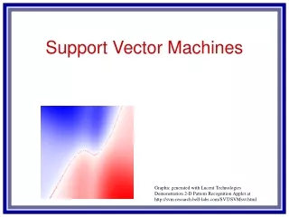
Cool Picture SVM A better example of what can happen by transforming to higher dimension
Feature Space SVM • Usually, higher dimension is bad news • From computational complexity POV • The so-called “curse of dimensionality” • But higher dimension feature space can make data linearly separable • Can we have our cake and eat it too? • Linearly separable and easy to compute • Yes, thanks to the kernel trick
Kernel Trick SVM • Enables us to work in input space • With results mapped to feature space • No work done explicitly in feature space • Computations in input space • Lower dimension, so computation easier • Results actually in feature space • Higher dimension, so easier to separate • Very cool trick!
Kernel Trick SVM • Unfortunately, to understand kernel trick, must dig a little (lot?) deeper • Also makes other aspects clearer • We won’t cover every detail here • Just enough to get idea across • Well, maybe a little more than that… • We need Lagrange multipliers • But first, constrained optimization
Constrained Optimization 4 2 f(x) 0 x = 1 -2 -4 -2 -1 1 2 0 SVM • “No brainer” example • Maximize: f(x) = 4 – x2 subject to x – 1 = 0 • Solution? • Max is at x = 1 • Max value is f(1) = 3 • Consider more general case next…
Lagrange Multipliers SVM • Maximize f(x,y) subject to g(x,y) = c • Define the Lagrangian L(x,y,λ) = f(x,y) + λ(g(x,y) – c) • “Stationary points” of L are possible solutions to original problem • All solutions must be stationary points • Not all stationary points are solutions • Generalize: More variables/constraints
Lagrangian SVM • Consider L(x,y,λ) = f(x,y) + λ(g(x,y) – c) • If g(x,y) = c, then constraint is satisfied and L(x,y,λ) = f(x,y) • Want to maximize over such (x,y) • If g(x,y) ≠ c then λ can “pull down” • Desired solution: max min L(x,y,λ) • Where max over (x,y) and min over λ
Lagrangian SVM • The Lagrangian is L(x,y,λ) = f(x,y) + λ(g(x,y) – c) • And max min L(x,y,λ) solves original constrained optimization problem • Therefore, solution to original problem is a saddle point of L(x,y,λ) • That is, max in one direction and min in the other example on next slide
Saddle Points SVM • Graph of L(x,λ) = 4-x2 +λ(x-1) • “No brainer” example from previous slide
Stationary Points SVM • Has nothing to do with fancy paper • That’s stationery, not stationary… • Stationary point means partial derivatives are all 0, that is dL/dx = 0 anddL/dy = 0 anddL/dλ = 0 • As mentioned, this generalizes to… • More variables in functions f and g • More constraints: Σλi (gi(x,y) – ci)
Another Example SVM • Lots of good geometric examples • We look at something different • Consider discrete probability distribution on n points: p1,p2,p3,…,pn • What distribution has max entropy? • Maximize entropy function • Subject to constraint that pj form a probability distribution
Maximize Entropy SVM • Shannon entropy: Σpj log2pj • Have a probability distribution, so… • Require 0 ≤ pj ≤ 1 for all j, and Σpj = 1 • We will solve this problem: • Maximize f(p1,..,pn) = Σpj log2pj • Subject to constraint Σpj = 1 • How should we solve this? • Do you really have to ask?
Entropy Example SVM • Recall L(x,y,λ) = f(x,y) + λ (g(x,y) – c) • Problem statement • Maximize f(p1,..,pn) = Σpj log2pj • Subject to constraint Σpj = 1 • In this case, Lagrangian is L(p1,…,pn,λ) = Σpj log2pj + λ (Σpj – 1) • Compute partial derivatives wrt each pj and partial derivative wrtλ
Entropy Example SVM • Have L(x,y,λ) = Σpj log2pj + λ (Σpj – 1) • Partial derivatives wrt any pj yields log2pj + 1/ln(2) + λ = 0 (#) • And wrtλ yields the constraint Σpj – 1 = 0 orΣpj = 1 (##) • Equation (#) implies all pj are equal • With equation (##), all pj = 1/n • Conclusion?
Notation SVM • Let x=(x1,x2,…,xn) and λ=(λ1,λ2,…,λm) • Then we write Lagrangian as L(x,λ) = f(x) + Σλi (gi(x) – ci) • Note: L is a function of n+m variables • Can view the problem as follows • The gi functions define a feasible region • Maximize f over this feasible region
Lagrangian Duality SVM • For Lagrange multipliers… • Primal problem: max min L(x,y,λ) • Where max over (x,y) and min over λ • Dual problem: min max L(x,y,λ) • As above, max over (x,y) and min over λ • In general, min max F(x,y,λ) ≥ max min F(x,y,λ) • But for L(x,y,λ), equality holds
Yet Another Example SVM Maximize: f(x,y) = 16 – (x2 + y2) Subject to: 2x – y = 4 Graph of f(x,y)
Intersection SVM Intersection of f(x,y) and 2x – y = 4 What is the solution to problem?
Primal Problem SVM • Maximize: f(x,y) = 16 – (x2 + y2) • Subject to: 2x – y = 4 • Then L(x,y,λ) = 16 – (x2 + y2) + λ(2x – y - 4) • Compute partial derivatives… dL/dx = -2x – 2λ = 0 dL/dy = -2y – λ = 0 dL/dλ = 2x – y – 4 = 0 • Result: (x,y,λ) = (-8/5,4/5,-8/5) • And f(x,y) = 64/5
Dual Problem SVM • Maximize: f(x,y) = 16 – (x2 + y2) • Subject to: 2x – y = 4 • ThenL(x,y,λ) = 16–(x2+y2)+λ(2x–y-4) • Recall that dual problem is min max L(x,y,λ) • Where max is over (x,y), min is over λ • How can we solve this?
Dual Problem SVM • Dual problem: min max L(x,y,λ) • So, can first take max of L over (x,y) • Then we are left with function L only in λ • To solve problem, find minL(λ) • On next slide, we illustrate this for L(x,y,λ) = 16 – (x2 + y2) + λ(2x – y - 4) • Same example as primal problem above
Dual Problem SVM • Given L(x,y,λ) = 16 – (x2 + y2) + λ(2x – y – 4) • Maximize over (x,y) by computing dL/dx = -2x + 2λ = 0 dL/dy = -2y - λ = 0 • Which implies x = λand y = -λ/2 • Substitute these into L to obtain L(λ) = 5/4λ2 + 4λ + 16
Dual Problem SVM • Original problem • Maximize: f(x,y) = 16 – (x2 + y2) • Subject to: 2x – y = 4 • Solution can be found by minimizing L(λ) = 5/4λ2 + 4λ + 16 • Then L’(λ) = 5/2λ + 4 = 0, which gives λ = -8/5 and (x,y) = (-8/5,4/5) • Same solution as the primal problem
Dual Problem SVM Maximize to find (x,y) in terms of λ Then rewrite L as function of λ only Finally, minimize L(λ) to solve problem But, why all of the fuss? Dual problem allows us to write the problem in more user-friendly way In SVM, we’ll make use of L(λ)
Lagrange Multipliers and SVM SVM • Lagrange multipliers very cool indeed • But what does this have to do with SVM? • Can view (soft) margin computation as constrained optimization problem • In this form, kernel trick will be clear • We can kill 2 birds with 1 stone • Make margin calculation clearer • Make kernel trick perfectly clear
Problem Setup SVM • Let X1,X2,…,Xn be data points • Each Xi = (xi,yi) a point in the plane • In general, could be higher dimension • Let z1,z2,…,zn be corresponding class labels, where each zi{-1,1} • Where zi = 1 if classified as “red” type • And zi = -1 if classified as “blue” type • Note that this is a binary classifier
Geometric View y x SVM • Equation of yellow line w1x + w2y + b = 0 • Equation of red line w1x + w2y + b = 1 • Equation of blue line w1x + w2y + b = -1 • Margin is distance between red and blue
Geometric View y x SVM • Any red point X=(x,y) must satisfy w1x + w2y + b ≥ 1 • Any blue point X=(x,y) must satisfy w1x + w2y + b ≤ -1 • Want inequalities all true after training
Geometric View y x SVM • With lines defined… • Given new data point X = (x,y) to classify • “Red” provided that w1x + w2y + b > 0 • “Blue” provided that w1x + w2y + b < 0 • This is scoring phase
Geometric View y x SVM • The real question is... • How to find equation of the yellow line? • Given {Xi} and {zi} • Where Xi point in plane • And zi its classification • Finding yellow line is the training phase…
Geometric View x m y SVM • Distance from origin to line Ax+By+C = 0 is |C| / sqrt(A2 + B2) • Origin to red line: |1-b| / ||W|| where W = (w1,w2) • Origin to blue line: |-1-b| / ||W|| • Margin is m = 2/||W||
Training Phase SVM • Given {Xi} and {zi}, find largest margin m that classifies all points correctly • That is, find red, blue lines in picture • Recall red line is of the form w1x + w2y + b = 1 • Blue line is of the form w1x + w2y + b = -1 • And maximize margin: m = 2/||W||
Training SVM • Since zi{-1,1}, correct classification occurs provided zi(w1xi + w2yi + b) ≥ 1 for all i • Training problem to solve: • Maximize: m = 2/||W|| • Subject to constraints: zi(w1xi + w2yi + b) ≥ 1 for i=1,2,…,n • Can we determine W and b ?
Training SVM • The problem on previous slide is equivalent to the following • Minimize: F(W) = ||W||2 / 2 = (w12 + w22) / 2 • Subject to constraints: 1 - zi(w1xi + w2yi + b) ≤ 0 for all i • Should be starting to look familiar…
Lagrangian SVM • Pretend inequalities are equalities… L(w1,w2,b,λ) = (w12 + w22) / 2 + Σ λi(1 - zi(w1xi + w2yi + b)) • Compute dL/dw1 = w1 - Σλizixi = 0 dL/dw2 = w2 - Σλiziyi = 0 dL/db = Σλizi= 0 dL/dλi = 1 - zi(w1xi + w2yi + b) = 0
Lagrangian SVM • Derivatives yield constraints and W = ΣλiziXiand Σλizi= 0 • Substitute these into L yields L(λ) = Σλi – ½ ΣΣλiλjzizjXiXj Where “” is dot product: XiXj= xixj+ yiyj • Here, L is only a function of λ • We still have the constraint Σλizi= 0 • Note: If we find λi then we know W