Support Vector Machines
420 likes | 707 Views
Support Vector Machines. Lecturer : Yishay Mansour Itay Kirshenbaum. Lecture Overview. In this lecture we present in detail one of the most theoretically well motivated and practically most effective classification algorithms in modern machine learning: Support Vector Machines (SVMs). .

Support Vector Machines
E N D
Presentation Transcript
Support Vector Machines Lecturer: Yishay Mansour Itay Kirshenbaum
Lecture Overview In this lecture we present in detail one of the most theoretically well motivated and practically most effective classification algorithms in modern machine learning: Support Vector Machines (SVMs).
Lecture Overview – Cont. • We begin with building the intuition behind SVMs • continue to define SVM as an optimization problem and discuss how to efficiently solve it. • We conclude with an analysis of the error rate of SVMs using two techniques: Leave One Out and VC-dimension.
Introduction • Support Vector Machine is a supervised learning algorithm • Used to learn a hyperplane that can solve the binary classification problem • Among the most extensively studied problems in machine learning.
Binary Classification Problem • Input space: • Output space: • Training data: • S drawn i.i.d with distribution D • Goal: Select hypothesis that best predicts other points drawn i.i.d from D
Binary Classification – Cont. • Consider the problem of predicting the success of a new drug based on a patient height and weight • m ill people are selected and treated • This generates m 2d vectors (height and weight) • Each point is assigned +1 to indicate successful treatment or -1 otherwise • This can be used as training data
Binary classification – Cont. • Infinitely many ways to classify • Occam’s razor – simple classification rules provide better results • Linear classifier or hyperplane • Our class of linear classifiers:
Choosing a Good Hyperplane • Intuition • Consider two cases of positive classification: • w*x + b = 0.1 • w*x + b = 100 • More confident in the decision made by the latter rather than the former • Choose a hyperplane with maximal margin
Good Hyperplane – Cont. • Definition: Functional margin S • A linear classifier:
Maximal Margin • w,b can be scaled to increase margin • sign(w*x + b) = sign(5w*x + 5b) for all x • (5w, 5b) is 5 times greater than (w,b) • Cope by adding an additional constraint: • ||w|| = 1
Maximal Margin – Cont. • Geometric Margin • Consider the geometric distance between the hyperplane and the closest points
Geometric Margin • Definition: • Definition: Geometric margin S • Relation to functional margin • Both are equal when
The Algorithm • We saw: • Two definitions of the margin • Intuition behind seeking a maximizing hyperplane • Goal: Write an optimization program that finds such a hyperplan • We always look for (w,b) maximizing the margin
The Algorithm – Take 1 • First try: • Idea • Maximize - For each sample the Functional margin is at least • Functional and geometric margin are the same as • Largest possible geometric margin with respect to the training set
The Algorithm – Take 2 • The first try can’t be solved by any off-the-shelf optimization software • The constraint is non-linear • In fact, it’s even non-convex • How can we discard the constraint? • Use geometric margin!
The Algorithm – Take 3 • We now have a non-convex objective function – The problem remains • Remember • We can scale (w,b) as we wish • Force the functional margin to be 1 • Objective function: • Same as: • Factor of 0.5 and power of 2 do not change the program – Make things easier
The algorithm – Final version • The final program: • The objective is convex (quadratic) • All constraints are linear • Can solve efficiently using standard quadratic programing (QP) software
Convex Optimization • We want to solve the optimization problem more efficiently than generic QP • Solution – Use convex optimization techniques
Convex Optimization – Cont. • Definition: A convex function • Theorem
Convex Optimization Problem • Convex optimization problem • We look for • a value of • Minimizes • Under the constraint
Lagrange Multipliers • Used to find a maxima or a minima of a function subject to constraints • Use to solve out optimization problem • Definition
Primal Program • Plan • Use the Lagrangian to write a program called the Primal Program • Equal to f(x) is all the constraints are met • Otherwise – • Definition – Primal Program
Primal Progam – Cont. • The constraints are of the form • If they are met • is maximized when all are 0, and the summation is 0 • Otherwise • is maximized for
Primal Progam – Cont. • Our convex optimization problem is now: • Define as the value of the primal program
Dual Program • We define the Dual Program as: • We’ll look at • Same as our primal program • Order of min / max is different • Define the value of our Dual Program
Dual Program – Cont. • We want to show • If we find a solution to one problem, we find the solution to the second problem • Start with • “max min” is always less then “min max” • Now on to
Dual Program – Cont. • Claim • Proof • Conclude
Karush-Kuhn-Tucker (KKT) conditions • KKT conditions derive a characterization of an optimal solution to a convex problem. • Theorem
KKT Conditions – Cont. • Proof • The other direction holds as well
KKT Conditions – Cont. • Example • Consider the following optimization problem: • We have • The Lagragian will be
Optimal Margin Classifier • Back to SVM • Rewrite our optimization program • Following the KKT conditions • Only for points in the training set with a margin of exactly 1 • These are the support vectors of the training set
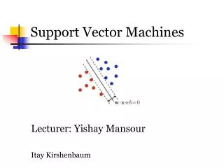
Optimal Margin – Cont. • Optimal margin classifier and its support vectors
Optimal Margin – Cont. • Construct the Lagragian • Find the dual form • First minimize to get • Do so by setting the derivatives to zero
Optimal Margin – Cont. • Take the derivative with respect to • Use in the Lagrangian • We saw the last tem is zero
Optimal Margin – Cont. • The dual optimization problem • The KKT conditions hold • Can solve by finding that maximize • Assuming we have – define • The solution to the primal problem
Optimal Margin – Cont. • Still need to find • Assume is a support vector • We get
Error Analysis Using Leave-One-Out • The Leave-One-Out (LOO) method • Remove one point at a time from the training set • Calculate an SVM for the remaining points • Test our result using the removed point • Definition • The indicator function I(exp) is 1 if exp is true, otherwise 0
LOO Error Analysis – Cont. • Expected error • It follows the expected error of LOO for a training set of size m is the same as for a training set of size m-1
LOO Error Analysis – Cont. • Theorem • Proof
Generalization Bounds Using VC-dimension • Theorem • Proof
Generalization Bounds Using VC-dimension – Cont. • Proof – Cont.
