Download
1 / 36
360 likes | 455 Views
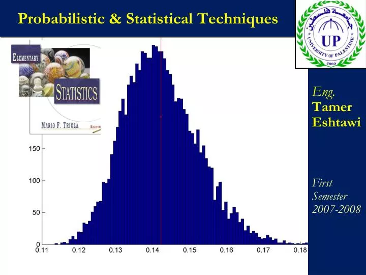
Probabilistic & Statistical Techniques. Eng. Tamer Eshtawi First Semester 2007-2008. Lecture 11. Chapter 6 (part 2) Normal Probability Distribution. Section 6-4 Sampling Distributions and Estimators. Key Concept.

E N D
Probabilistic & Statistical Techniques Eng. Tamer Eshtawi First Semester 2007-2008
Lecture 11 Chapter 6 (part 2)Normal Probability Distribution Main Reference: Pearson Education, Inc Publishing as Pearson Addison-Wesley.
Section 6-4 Sampling Distributions and Estimators
Key Concept The main objective of this section is to understand the concept of a sampling distribution of a statistic, which is the distribution of all values of that statistic when all possible samples of the same size are taken from the same population. We will also see that some statistics are better than others for estimating population parameters.
Definition • The sampling distribution of a statistic • (such as the sample mean) is the distribution of all values of the statistic when all possible samples of the same size n are taken from the same population. Population Sample Size n Sample Size n Sample Size n
Properties • Sample proportions tend to target the value of the population proportion. (That is, all possible sample proportions have a mean equal to the population proportion.) • Under certain conditions, the distribution of the sample proportion can be approximated by a normal distribution.
Estimators Some statistics work much better than others as estimators of the population. The example that follows shows this:
Example - Sampling Distributions A population consists of the values 1, 2, and 5. We randomly select samples of size 2with replacement. There are 9 possible samples. a. For each sample, find the mean, median, range, variance, and standard deviation. b. For each statistic, find the mean from part (a)
Interpretation of Sampling Distributions We can see that when using a sample statistic to estimate a population parameter, some statistics are good in the sense that they target the population parameter and are therefore likely to yield good results. Such statistics are called unbiased estimators. Statistics that target population parameters: mean, variance, proportion Statistics that do not target population parameters: median, range, standard deviation
Section 6-5 The Central Limit Theorem
Key Concept The procedures of this section form the foundation for estimating population parameters and hypothesis testing – topics discussed at length in the following chapters.
Central Limit Theorem Given: • The random variable x has a distribution (which may or may not be normal) with mean µ and standard deviation . 2. Simple random samples all of size nare selected from the population. (The samples are selected so that all possible samples of the same size n have the same chance of being selected.)
Central Limit Theorem Conclusions: 1. The distribution of sample mean will, as the sample size increases, approach a normal distribution. 2. The mean of the sample means is the population mean µ. 3. The standard deviation of all sample means is
Practical Rules Commonly Used • For samples of size nlarger than 30, the distribution of the sample means can be approximated reasonably well by a normal distribution. The approximation gets better as the sample size n becomes larger. 2. If the original population is itself normally distributed, then the sample means will be normally distributed for any sample size n (not just the values of n larger than 30).
Notation the mean of the sample means the standard deviation of sample mean (often called the standard error of the mean)
Simulation With Random Digits Generate 500,000 random digits, group into 5000 samples of 100 each. Find the mean of each sample. Even though the original 500,000 digits have a uniform distribution, the distribution of 5000 sample means is approximately a normal distribution!
Important Point As the sample size increases, the sampling distribution of sample means approaches a normal distribution.
Example – Water Taxi Safety Given the population of men has normally distributed weights with a mean of 172 lb and a standard deviation of 29 lb, a) if one man is randomly selected, find the probability that his weight is greater than 175 lb.b) if 20 different men are randomly selected, find the probability that their mean weight is greater than 175 lb (so that their total weight exceeds the safe capacity of 3500 pounds).
Example – cont a) if one man is randomly selected, find the probability that his weight is greater than 175 lb. P ( x > 174 lb.) = 1- P(x < 174) 1- P(z < 0.1) = 1- 0.5398=0.4602
Example – cont b) if 20 different men are randomly selected, find the probability that their mean weight is greater than 175 lb.
b) if 20 different men are randomly selected, their mean weight is greater than 175 lb.P(x > 175) = 0.3228 Example - cont a) if one man is randomly selected, find the probability that his weight is greater than 175 lb.P(x > 175) = 0.4602 It is much easier for an individual to deviate from the mean than it is for a group of 20 to deviate from the mean.
Interpretation of Results Given that the safe capacity of the water taxi is 3500 pounds, there is a fairly good chance (with probability 0.3228) that it will be overloaded with 20 randomly selected men.
finite population correction factor Correction for a Finite Population When sampling without replacement and the sample size nis greater than 5% of the finite population of size N, adjust the standard deviation of sample means by the following correction factor:
Section 6-7 Assessing Normality
Key Concept This section provides criteria for determining whether the requirement of a normal distribution is satisfied. The criteria involve visual inspection of a histogram to see if it is roughly bell shaped, identifying any outliers, and constructing a new graph called a normal quantile plot.
Definition Anormal quantile plot (ornormal probability plot) is a graph of points (x,y), where each x value is from the original set of sample data, and each y value is the corresponding z score that is a quantile value expected from the standard normal distribution.
Methods for Determining Whether Data Have a Normal Distribution 1. Histogram:Construct a histogram. Reject normality if the histogram departs dramatically from a bell shape. 2. Outliers:Identify outliers. Reject normality if there is more than one outlier present. 3. normal probability plot : If the histogram is basically symmetric and there is at most one outlier, construct a normal probability plot as follows:
Procedure for Determining Whether Data Have a Normal Distribution - cont a. Sort the data by arranging the values from lowest to highest. b. With a sample size n, each value represents a proportion of 1/n of the sample. Using the known sample size n, identify the areassuch as 1/2n, 3/2n, 5/2n, 7/2n, and so on.These are the cumulative areas to the left of the corresponding sample values. c. Use the standard normal distribution (Table A-2, software or calculator) to find the z scores corresponding to the cumulative left areas found in Step (b). 3. Normal probability plot
Procedure for Determining Whether Data Have a Normal Distribution - cont d. Plot the points (x, y), where each x is an original sample value and y is the correspondingzscore. e. Examine the normal quantile plot using these criteria: If the points do not lie close to a straight line, then the data appear to come from a population that does not have a normal distribution. If the pattern of the points is reasonably close to a straight line, then the data appear to come from a population that has a normal distribution.
Example Interpretation: Because the points lie reasonably close to a straight line and there does not appear to be a systematic pattern that is not a straight-line pattern, we conclude that the sample appears to be a normally distributed population.
Example Check whether the requirement of a normal distribution is satisfied or not in the following data