The R-matrix Method for oriented molecules
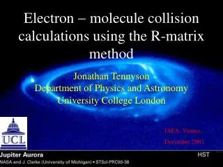
The R-matrix Method for oriented molecules. e -. Jonathan Tennyson University College London. Jonathan Tennyson Department of Physics and Astronomy University College London. Outer region. Inner region. UCL, May 2004. Montreal Oct 2009. Lecture course on open quantum systems.
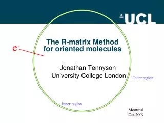

The R-matrix Method for oriented molecules
E N D
Presentation Transcript
The R-matrix Methodfor oriented molecules e- Jonathan Tennyson University College London Jonathan Tennyson Department of Physics and Astronomy University College London Outer region Inner region UCL, May 2004 Montreal Oct 2009 Lecture course on open quantum systems
What is an R-matrix? Consider coupled channel equation: Use partial wave expansion hi,j(r,q,f) = Plm (q,f) uij(r) Plm associated Legendre functions where General definition of an R-matrix: where b is arbitrary, usually choose b=0.
R-matrix propagation Asymptotic solutions have form: open channels closed channels R-matrix is numerically stable For chemical reactions can start from Fij = 0 at r = 0 Light-Walker propagator: J. Chem. Phys. 65, 4272 (1976). Also: Baluja, Burke & Morgan, Computer Phys. Comms., 27, 299 (1982) and 31, 419 (1984).
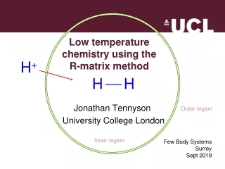
Wigner-Eisenbud R-matrix theory Outer region e- H H Inner region R-matrix boundary
Consider the inner region Schrodinger Eq: Finite region introduces extra surface operator: Bloch term: for spherical surface at r = x; b arbitrary. Necessary to keep operator Hermitian. Schrodinger eq. for finite volume becomes: which has formal solution
Eq. 1 Expand u in terms of basis functions v Coefficients aijkdetermined by solving Inserting this into eq. 1 Eq. 2
R-matrix on the boundary Eq. 2 can be re-written using the R-matrix which gives the form of the R-matrix on a surface at r = x: in atomic units, where Ek is called an ‘R-matrix pole’ uik is the amplitude of the channel functions at r = x.
Why is this an “R”-matrix? In its original form Wigner, Eisenbud & others used it to characterise resonances in nuclear reactions. Introduced as a parameterisation scheme on surface of sphere where processes inside the sphere are unknown.
Resonances:quasibound states in the continuum • Long-lived metastable state where the scattering electron is temporarily captured. • Characterised by increase in p in eigenphase. • Decay by autoionisation (radiationless). • Direct & Indirect dissociative recombination (DR), and other processes, all go via resonances. • Have position (Er) and width (G) (consequence of the Uncertainty Principle). • Three distinct types in electron-molecule collisions: Shape, Feshbach & nuclear excited.
Electron – molecule collisions Outer region e- H H Inner region R-matrix boundary
Dominant interactions Inner region Exchange Correlation Adapt quantum chemistry codes High l functions required Integrals over finite volume Include continuum functions Special measures for orthogonality CSF generation must be appropriate Boundary Target wavefunction has zero amplitude Outer region Adapt electron-atom codes Long-range multipole polarization potential Many degenerate channels Long-range (dipole) coupling
Inner region: Scattering wavefunctions Yk= A Si,jai,j,k fiN hi,j + Sm bm,kfmN+1 where fiN N-electron wavefunction of ith target state hi,j1-electron continuum wavefunction fmN+1 (N+1)-electron short-range functions ‘L2’ ai,j,kand bj,kvariationally determined coefficients AAntisymmetrizes the wavefunction
Target Wavefunctions fiN = Si,j ci,jzj where fiN N-electron wavefunction of ith target state zjN-electron configuration state function (CSF) Usually defined using as CAS-CI model. Orbitals either generated internally or from other codes ci,jvariationally determined coefficients
Use partial wave expansion (rapidly convergent) hi,j(r,q,f) = Plm (q,f) uij(r) Plm associated Legendre functions Continuum basis functions • Diatomic code: l any, in practice l < 8 u(r) defined numerically using boundary condition u’(r=a) = 0 This choice means Bloch term is zero but Needs Buttle Correction…..not strictly variational Schmidt & Lagrange orthogonalisation • Polyatomic code: l < 5 u(r) expanded as GTOs No Buttle correction required…..method variational But must include Bloch term Symmetric (Lowden) orthogonalisation Linear dependence always an issue
R-matrix wavefunction Yk= A Si,jai,j,k fiN hi,j + Smbm,k fmN+1 only represents the wavefunction within the R-matrix sphere ai,j,kand bj,kvariationally determined coefficients by diagonalising inner region secular matrix. Associated energy (“R-matrix pole”) is Ek. Full, energy-dependent scattering wavefunction given by Y(E) = SkAk(E) Yk Coefficients Ak determined in outer region (or not) Needed for photoionisation, bound states, etc. Numerical stability an issue.
Propagate R-matrix (numerically v. stable) R-matrix outer region:K-, S- and T-matrices Asymptotic boundary conditions: Open channels Closed channels Defines the K (“reaction”)-matrix. K is real symmetric. Diagonalising K KD gives the eigenphase sum Use eigenphase sum to fit resonances Eigenphase sum The K-matrix can be used to define the S (“scattering”) and T (“transition”) matrices. Both are complex. , T = S-1 Use T-matrices for total and differential cross sections S-matrices for Time-delays & MQDT analysis
UK R-matrix codes: www.tampa.phys.ucl.ac.uk/rmat SCATCI: Special electron Molecule scattering Hamiltonian matrix construction L.A. Morgan, J. Tennyson and C.J. Gillan, Computer Phys. Comms., 114, 120 (1999).
Processes: at low impact energies Elastic scattering AB + e AB + e Electronic excitation AB + e AB* + e Vibrational excitation AB(v”=0) + e AB(v’) + e Rotational excitation AB(N”) + e AB(N’) + e Dissociative attachment / Dissociative recombination AB + e A + B A + B Impact dissociation AB + e A + B + e All go via (AB-)** . Can also look for bound states
Adding photons I. Weak fields d s = 4 p2 a a02 w | <FE(-) | m | F0>|2 dW Atoms: Burke & Taylor, J Phys B, 29, 1033 (1975) Molecules: Tennyson, Noble & Burke, Int. J. Quantum Chem, 29, 1033 (1986)
II. Intermediate fields R-matrix – Floquet Method Inner region Hamiltonian: linear molecule, parallel alignment Colgan et al, J Phys B, 34, 2084 (2001)
III. Strong Fields Time-dependent R-matrix method: Theory: Burke & Burke, J Phys B, 30, L380 (1997) Atomic implementation: Van der Hart, Lysaght & Burke, Phys Rev A 76, 043405 (2007) Atoms & molecules: numerical procedure Lamprobolous, Parker & Taylor, Phys Rev A, 78, 063420 (2008) Molecular implementation: awaited
Molecular alignment: Alex Harvey Harvey & Tennyson J. Mod Opt. 54, 1099 (2007) Harvey & Tennyson J.Phys. B. 42, 095101 (2009) • No Laser field. • Re-scattering = scattering from molecular cation. • Nuclei fixed at neutral molecules geometry • Energy range up to ionisation potential of the cation (2nd ionisation potential of the molecule) • Relevant excited states included in calculations • Initially looked at parallel alignment and elastic scattering. • Total scattering symmetry 1Σg+ and 1Σu+
Parallel Alignment • Dipole selection rules and linearly polarised light. Molecule starts in ground state (aligned parallel to polarisation) • Odd number of photons 1Σg+ 1Σu+ transition • Even number of photons 1Σg+1Σg+ transition
Results: H2 Total Cross Sections • Close coupling expansion: 3 lowest ion states • Aligned xsec 3 to 4 times larger • Simplistic explanation: for 2Σg+ ground state electron takes longer path through molecule – more chance to interact
Energies below 1st resonance • 1Σu+: no shape change. • 1Σg+: Strong forward and backwards scattering Differential cross section against scattering angle (3-9eV) Top: Orientationally averaged, Bottom: parallel aligned, Left: 1Σg+, Right: 1Σu+ H2 : Differential Cross Sections: low energies
Differential cross section against scattering angle (15.5-21eV) Left: 1Σg+, Right: 1Σu+ H2 : Differential Cross Sections: higher energies • Energies above first resonance ~13eV and 1st threshold ~18eV. • 1Σg+ Inversion for DCS between first and second resonance.
H2 : Total Xsec as a function of alignment Note: For non-parallel alignments need to consider other symmetries but for 2Σg+ ground state we expect the contribution to be minor. Total cross section as a function of alignment angle β; Left: 1Σg+, Right: 1Σu+
CO2 : Total xsec as a function of alignment • 3 state model: couples ion X, A and B states • Zero xsec for parallel alignment! Due to 2Πg ground state • Other symmetries important, e.g. expect Π total symmetry to be dominant at low energy as it couples to σ-continuum • 1Σg+ peaks 50-55° deg and 125-130° • 1Σu+ peaks 90°, 35-40° and 140-145° Experimental HHG intensity against alignment. Mairesse et al. J. Mod. Opt. 55 16 (2008) 1Σg+ 1Σu+ Total cross section as a function of alignment angle β
Differential Cross Section: Polar Plots Calculations neglect the Coulomb phase 1Σg+ 1Σu+ Polar plots of the differential cross section as a function of scattering angle at 3eV, β = 30°; in the z-x plane; r = DCS, θ = scattering angle
Differential Cross Section: Polar Plots 1Σg+ 1Σu+ Polar plots of the differential cross section as a function of scattering angle at 3 eV, β = 30°; in the z-x plane; r = DCS, θ = scattering angle No Coulomb phase With Coulomb phase
Future Work • Effect of adding more scattering symmetries. • Inelastic cross sections. • Extended energy range: RMPS method. • Incorporate scattering amplitudes into a strong field model. • Issues with treatment of Coulomb phases