Download

1 / 25
250 likes | 291 Views
Explore the Bayesian biosurveillance goals and PANDA model for rapid outbreak detection, identifying affected individuals, and predicting at-risk populations using causal Bayesian networks. Learn how Bayesian inference aids in modeling an entire population for biosurveillance. Discover the evaluation results of PANDA's spatial model and optimized versions compared to control chart methods. Uncover the potential of causal networks in biosurveillance and the future work involving modeling contagious diseases, integrating over-the-counter data, and enhancing alert systems with realistic decision models and explanations.

E N D
Bayesian Biosurveillance of Disease Outbreaks Gregory F. Cooper, Denver H. Dash, John D. Levander, Weng-Keen Wong, William R. Hogan, Michael M. Wagner RODS Laboratory Center for Biomedical Informatics University of Pittsburgh
Outline • Biosurveillance goals • Bayesian biosurveillance • A Bayesian biosurveillance model (PANDA) • Summary and future plans
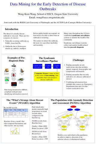
Biosurveillance Detection Goals • Detect an unanticipated biological disease outbreak in the population as rapidly and as accurately as possible • Determine the people who already have the disease • Predict the people who are likely to get the disease
PANDA: Population-wide ANomaly Detection and Assessment • PANDA models outbreaksusing a causal Bayesian network. • The causal Bayesian network in PANDA represents probabilistic causal relationships that link outbreak etiologies to available evidence, such as emergency department (ED) visits. • The network is assessed from training data and from knowledge of outbreak disease from the literature.
Example of a PANDA Bayesian Network that Models a Disease Outbreak Due to an AirborneRelease of Anthrax Global nodes Person model G Interface nodes P4 I P1 P2 P3
The probabilities in the person-network models were estimated from U.S. Census data, from historical ED data from Allegheny county, and from the anthrax literature. The population currently being modeled consists of all ~1.4M people in Allegheny County The smallest region modeled is a Zip code, and all Zip codes in Allegheny county are included. Some Current Model Details
Equivalence Classes The 1.4M people in the modeled population can be partitioned into approximately 48,000 equivalence classes
Define the background population (e.g., using census data) As patients enter the ED, they get moved from their background class to a patient class corresponding to their symptoms. After sufficient time passes, patients get moved back into their background class, while other patients get added. Modeling an Entire Population people not seen in the ED people seen in the ED
Tractably Modeling an Entire Population Pre-compute the probability of observing the entire background population, and replace all equivalence classes with a single (binary) master node:
Simple Adjustment Rule As a person moves from equivalence class Ei to class Ej, we can easily adjust the probability table of E to reflect the change using:
For testing, an outdoor anthrax release was simulated using the anthrax cases output by the BARD system. The BARD-simulated cases of infected individuals who visited the ED were overlaid onto actual historical ED data. Ninety-six such scenarios were generated and for each the data stream of ED cases was given as input to PANDA. Each simulated hour, PANDA generated a posterior probability of an anthrax outbreak. We plotted time-to-detection versus the false-positive rate of detection. Evaluation
Timing Results The following timing results are based on monitoring historical ED data over six days using PANDA running on an AMD Opteron 248 (2.19 GHz and 4 GB RAM). Original Model:4 to 5 seconds of machine time Original Model with Season, Day of Week, Time of Day: 15 seconds Spatial Model: 20 seconds Spatial Model with Season, Day of Week, Time of Day: 52 seconds
Summary • Biosurveillance can be viewed as ongoing diagnosis of an entire population. • Causal networks provide a flexible and expressive means of coherently modeling a population in performing biosurveillance. • Inference on causal networks can derive the type of posterior probabilities needed for biosurveillance. • Initial results from a simulation study are promising, but preliminary. • Inference can be computationally tractable when modeling non-contagious disease outbreaks, such as an outbreak due to the outdoor release of anthrax spores.
Future Work Includes … • Modeling contagious diseases • Including over-the-counter (OTC) data • Constructing realistic decision models about when to raise an alert • Developing explanations of alerts • Performing additional evaluations
Thank you RODS Laboratory: http:/www.health.pitt.edu/rods/ Bayesian Biosurveillance: http://www.cbmi.pitt.edu/panda/