Estimating a VAR

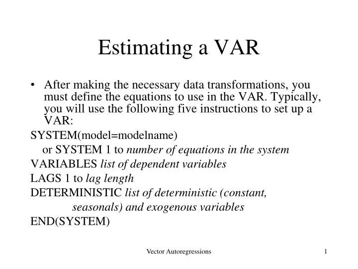
1. Estimating a VAR • After making the necessary data transformations, you must define the equations to use in the VAR. Typically, you will use the following five instructions to set up a VAR: SYSTEM(model=modelname) or SYSTEM 1 to number of equations in the system VARIABLES list of dependent variables LAGS 1 to lag length DETERMINISTIC list of deterministic (constant, seasonals) and exogenous variables END(SYSTEM) Vector Autoregressions

2. Example for estimating a VAR As illustrated in the Programming Manual, you can set up a 3-variable VAR for the variables dlrgdp, dlrm2, and drs using: system(model=var1) var dlrgdp dlrm2 drs lags 1 to 12 det constant end(system) The SYSTEM and VARIABLES (i.e., var) instructions set us a system of VAR equations called var1. Here the lag length is 12 and each regression equation includes a constant. Next, use ESTIMATE to obtain the results, save the residuals in the series resids12, and to save the variance/covariance matrix in V estimate(residuals=resids12,outsigma=V) Vector Autoregressions

3. Creating Seasonals ENTRY DECEMBER 1972:01 0 1972:02 0 1972:03 0 1972:04 0 1972:05 0 1972:06 0 1972:07 0 1972:08 0 1972:09 0 1972:10 0 1972:11 0 1972:12 1 cal 1972 1 12 all 1999:10 open data f:\classes\413\2000\cars.txt data(format=prn,org=obs) / seasonal december pri / december lin cars # constant december{0 to –10} Vector Autoregressions

4. estimate(OUTSIGMA=V,other options) start end residuals where: start end The range of entries to use. residuals The residuals from the first equation are stored in the series given by residuals, the residuals from the second equation are stored in series number residuals+1, and so forth. The appropriate number of series should be declared on the ALLOCATE instruction. OUTSIGMA= The name of the variance/covariance matrix. This option computes and saves the covariance matrix of the residuals. You must use this option if you want to perform innovation accounting or hypothesis tests The other principal options are: NOPRINT By default, RATS prints out the results of the OLS estimation of each equation. Use NOPRINT to suppress the output. NOFTESTS By default, RATS prints the results of all Granger causality tests. Use to supress this output. SIGMA This option computes and displays (but does not save) the covariance matrix of the residuals. Use both OUTSIGMA= and SIGMA if you want to compute, save, and print the variance/covariance matrix. Vector Autoregressions

5. Impulse Responses and Variance Decompositions errors(IMPULSES) equations steps name where: equations Number of equations in the VAR. steps The forecast horizon and the number of impulse responses. name The name of the covariance matrix used on the ESTIMATE instruction. The principal option is IMPULSES. If you exclude IMPULSES, RATS calculates and prints only the variance decompositions. There is a supplementary card for each equation Vector Autoregressions

6. Hypothesis Testing in RATS ratio(degrees=df ,mcorr=c,other options) start end # 1 2 ... n # n+1 n+2 ... 2n where: start end The range over which the test is to be performed. degrees= The number of degrees of freedom (equal to the number of restrictions in the system). mcorr= Sims= small sample correction for likelihood ratio tests (i.e., the value of c). Set mcorr equal to the largest number of parameters estimated in any one of the equations (usually equal to the number of parameters estimated in each of the unrestricted equations). NOPRINT, supresses the printing of the covariance matrices and the marginal significance level of the test. It is possible to obtain the marginal significance level with the instruction:  display %signif Vector Autoregressions

7. Example of a Cross Equation Restriction Example: Suppose, a two-variable VAR using 12 lags of each variable is estimated and the residuals are saved in series 1 and 2. The estimation is over the sample period 63:2 to 91:4. Next, the same sample period is used to estimate a model with a lag length of 8 and the residuals are saved in series 3 and 4. The lag length test is conducted using:  ratio(degrees=16,mcorr=28) 63:2 91:4 # 1 2 # 3 4 Vector Autoregressions

8. Multivariate AIC and SBC When you use the OUTSIGMA= option on the ESTIMATE statement, RATS computes the covariance matrix of the residuals. You can fetch the logarithmic determinant of this covariance matrix using %LOGDET. compute aic = %nobs*%logdet + 2*N compute sbc = %nobs*%logdet + N*log(%nobs) display ‘aic =‘ aic ‘sbc =‘ sbc where you must set N equal to the number of parameters estimated in the entire system Vector Autoregressions

9. Seemingly Unrelated Regressions Different lag lengths yt = a11(1)yt-1 + a11(2)yt-2 + a12zt-1 + e1t zt = a21yt-1 + a22zt-1 + e2t Non-Causality yt = a11yt-1 + e1t zt = a21yt-1 + a22zt-1 + e2t Effects of a third variable yt = a11yt-1 + a12zt-1 + e1t zt = a21yt-1 + a22zt-1 + a23wt + e2t Vector Autoregressions

10. Estimating a Near-VAR Step 1: As in Step 1 of a VAR estimation, use the ALLOCATE instruction to reserve room for each of the residual series. Step 2: You must define the equations to use in the near-VAR. The simplest way is to use the DEFINE= option of the LINREG instruction. To set up the first near-VAR system above, use: linreg(define=1) y # y{1 to 2} z{1} linreg(define=2) z # y{1} z{1} To set up the third near-VAR system above, use: linreg(define=1) y # y{1} z{1} linreg(define=2) z # y{1} z{1} w Vector Autoregressions

11. Near-VAR II Step 3 The typical syntax of SUR is: sur(options) equations start end # equation resids where: equations The number of equations in the system start end The range of entries to use. equation The number of the equation. resids The series in which to store the residuals. There is 1 supplementary instruction for each equation. Vector Autoregressions