Download

1 / 28
290 likes | 311 Views
This study compares coverage of CAPE vs. LFA LTG to create WRF forecasts of lightning threat based on simulated convection. It provides a calibrated threat for accurate flash rate densities and a robust algorithm for proxy data use. The methodology involves a blended threat constructed from LTG data and offers advantages and disadvantages. Finally, the study presents findings and insights from LFA studies using NSSL WRF output data.

E N D
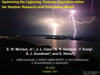
Optimization of the WRF Lightning Forecast Algorithm E. W. McCaul, Jr.1, J. L. Case2, S. R. Dembek1, F. Kong3, S. J. Goodman4, and S. Weiss5 USRA Huntsville; 2. ENSCO NASA SPoRT; 3. Univ. of Oklahoma; 4. NOAA/NESDIS; 5. NOAA/SPC WoF Workshop February, 2012 Photo, David Blankenship Guntersville, Alabama
LFA Objectives Given LTG link to large ice, and a cloud-scale model like WRF, which prognoses hydrometeors, LFA seeks to: Create WRF forecasts of LTG threat (1-36 h), based on simple proxy fields from explicitly simulated convection Construct a calibrated threat that yields accurate quantitative peak flash rate densities for the strongest storms, based on LMA total LTG observations 3. Provide robust algorithm for use in making proxy LTG data, and for potential uses with DA
Calibration Curve LTG1 (FLX) Units of F1 are fl/km2/5 min F1 = 0.042 FLX F1 > 0.01 r = 0.67
Calibration Curve LTG2 (VII) F2 = 0.2 VII Units of F2 are fl/km2/5 min F2 > 0.4 r = 0.83
Construction of blended threat:1. LTG1 and LTG2 are both calibrated to yield correct peak flash densities2. The peaks of LTG1 and LTG2 also tend to be coincident in all simulated storms, but LTG2 covers more area3. Thus, weighted linear combinations of the 2 threats will also yield the correct peak flash densities 4. To preserve most of time variability in LTG1, use large weight w15. To preserve areal coverage from LTG2, avoid very small weight w26. Tests using 0.95 for w1, 0.05 for w2, yield satisfactory results7. Thus, set LTG3 = 0.95*LTG1 + 0.05*LTG2
Methods based on LTG physics; should be robust and regime-independent Can provide quantitative estimates of flash rate fields; use of thresholds allows for accurate threat areal coverage Methods are fast and simple; based on fundamental model output fields; no need for complex electrification modules LTG Threat Methodology: Advantages
Methods are only as good as the numerical model output; models usually do not make storms in the right place at the right time; models sometimes do bad forecasts; saves at >5 min can miss LTG jumps Small number of cases, lack of extreme LTG events means uncertainty in calibrations Calibrations should be redone whenever model is changed, or error bars acknowledged regarding sensitivities to grid mesh, model microphysics (to be addressed here and in future) LTG Threat Methodology: Disadvantages
2-km horizontal grid mesh 51 vertical sigma levels Dynamics and physics: Eulerian mass core Dudhia SW radiation RRTM LW radiation YSU PBL scheme Noah LSM WSM 6-class microphysics scheme (graupel; no hail) 8h forecast initialized at 00 UTC with AWIP212 NCEP EDAS analysis; Also used METAR, ACARS, and WSR-88D radial vel at 00 UTC; Eta 3-h forecasts used for LBCs WRF Configuration (LFA study)Typical Case
4-km horizontal grid mesh 35 vertical sigma levels Dynamics and physics: Eulerian mass core Dudhia SW radiation RRTM LW radiation MYJ PBL scheme Noah LSM WSM 6-class microphysics scheme (graupel; no hail) 36h forecast initialized at 00 UTC with AWIP212 NCEP EDAS analysis on 40 km grid; 0-36-h NAM forecasts used for LBCs WRF Configuration (NSSL)Typical Case
Sample of NSSL WRF output, 20101130 (see www.nssl.noaa.gov/wrf)
Scatterplot of selected NSSL WRF output for LTG1, LTG2 (internal consistency check) Threats 1, 2 should cluster along diagonal; deviation at high flash rates indicates need to check calibration
Recent LFA studies, NSSL WRF, 2010-2011:(examined to test robustness in larger sample of model runs)1. Obtained NSSL WRF daily output for full 2010-2011 for three regions: HUN, OUN, USA2. HUN region examined (preliminary)3. OUN, USA regions to be examined soon4. May consult DCLMA because of OKLMA downtime issues5. Metric used in statistics scoring: did LTG occur in WRF LFA and/or in LMA obs, within the regions, in 0-24 h periods?6. Preliminary inspection of results shows: -frequent spurious activation of LFA in wintertime stratiform -occasional divergent LTG1, LTG2 values in high FRD cases, with LTG1 always > LTG2 (should be equal)7. Thus: need to reevaluate LFA for very low, very highFRDs
Recent LFA studies, NSSL WRF, 2010-2011:(examined to test robustness in larger sample of model runs) Preliminary findings for winter weather, JFMD2010,JFM20111. HUN region examined only (others to be examined later) 2. First findings, for winter weather (very low FRDs): - LFA produces 77 d of false alarms from LTG2 - LFA gives only 40 d of false alarms from LTG1 - no TSSN hits in HUN 2010; one in Jan 2011 (LTG1,LTG2) - if require LTG1>0.01, could reduce winter FA d by ~50% - if require LTG1>1.5, reduce FA d from 40 to 6 (85%) - use of LTG1 threshold too large might adversely affect deep convection; 3 of 6 FA events are for sleet, and these kinds of FA are impractical to eradicate
Recent LFA studies, NSSL WRF, 2010-2011: Contingency table findings for HUN winter stratiform weather format: n(JFMD2010) + n(JFM2011) = total uses LTG1 threshold = 0.01 fl km-2/(5 min) hit days | false alarm days | 0 + 1 = 1 | 23 + 17 = 40 | ------------------------------------------------------------------------- miss days | true null days | 0 + 0 = 0 | 75 + 43 = 118 |
Recent LFA studies, NSSL WRF, 2010-2011: Contingency table findings for HUN winter stratiform weather format: n(JFMD2010) + n(JFM2011) = total uses LTG1 threshold = 1.50 fl km-2/(5 min) hit days | false alarm days | 0 + 1 = 1 | 3 + 3 = 6 | ------------------------------------------------------------------------- miss days | true null days | 0 + 0 = 0 | 95 + 57 = 152 |
Recent LFA studies, NSSL WRF, 2010-2011: Contingency table findings for HUN winter stratiform weather (HUN area: 32.3<lat<36.7; -91.6<lon<-82.1)- winter stratiform regimes are dominated by large WRF bias; many low-grade false alarms, but few “hits,” and no “misses”- using forecast day-scale performance as the metric, we find:LTG1>0.01: LTG1>1.50: POD = 1.00 POD = 1.00 FAR = 0.98 FAR = 0.86 CSI = 0.02 CSI = 0.14 BIAS = 41.0 BIAS = 7.0 TSS = 0.75 TSS = 0.96 HSS = 0.04 HSS = 0.24Increasing the LTG1 threshold helps, but rarity of hits a problem
Recent LFA studies, NSSL WRF, 2010-2011:(examined to test robustness in larger sample of model runs) Preliminary findings for convective weather, JJA 2010-20111. HUN region examined only (others to be examined later) 2. First findings, for convective weather in HUN region, regarding general statistical behavior of LFA: - WRF has spinup problems in hours 0-4; exclude them - To eliminate double-counting, exclude WRF data after 24h - WRF output missing on 3 of 184 days in JJA 2010-11 - WRF predicts LTG in HUN for all 181 days in JJA 2010-11 - LMA observes LTG in HUN for 169 days in JJA 2010-11 - LFA produces only 11 d of false alarms (FAR=0.07) - LFA produces zero false null (miss) days (POD=1.00) - LFA has more false alarm days in transitional months
Recent LFA studies, NSSL WRF, 2010-2011: Contingency table findings for HUN convective weather format: n(JJA2010) + n(JJA2011) = total uses LTG1 threshold = 0.01 fl km-2/(5 min) hit days | false alarm days | 86 + 83 = 169 | 3 + 8 = 11 | ------------------------------------------------------------------------- miss days | true null days | 0 + 0 = 0 | 0 + 1 = 1 |
Recent LFA studies, NSSL WRF, 2010-2011: Contingency table findings for HUN convective weather format: n(JJA2010) + n(JJA2011) = total uses LTG1 threshold = 1.50 fl km-2/(5 min) hit days | false alarm days | 86 + 83 = 169 | 3 + 6 = 9 | ------------------------------------------------------------------------- miss days | true null days | 0 + 0 = 0 | 0 + 3 = 3 |
Recent LFA studies, NSSL WRF, 2010-2011: Contingency table findings for HUN convective weather (HUN area: 32.3<lat<36.7; -91.6<lon<-82.1)- convective regimes are dominated by large WRF hit rate; few false alarms, but some are big; again no “misses”- using forecast day-scale performance as the metric, we find:LTG1>0.01: LTG1>1.50: POD = 1.00 POD = 1.00 FAR = 0.07 FAR = 0.05 CSI = 0.94 CSI = 0.95 BIAS = 1.07 BIAS = 1.05 TSS = 0.08 TSS = 0.25 HSS = 0.15 HSS = 0.38Increasing the LTG1 threshold helps, but rarity of nulls a problem
Recent LFA studies, NSSL WRF, 2010-2011: Contingency table findings for HUN Springtime weather (HUN area: 32.3<lat<36.7; -91.6<lon<-82.1)- Spring (AM) convective regimes feature large WRF hit rate; some nulls and false alarms; again no “misses”- using forecast day-scale performance as the metric, we find:LTG1>0.01: LTG1>1.50: POD = 1.00 POD = 1.00 FAR = 0.28 FAR = 0.21 CSI = 0.72 CSI = 0.79 BIAS = 1.39 BIAS = 1.27 TSS = 0.42 TSS = 0.60 HSS = 0.46 HSS = 0.65Increasing the LTG1 threshold helps, but scores already good
Convective regimes - predictability:1. Stratify convective cases as supercell or multicell; 2. Supercell cases well handled quantitatively by LFA;3. Multicell cases are predicted by LFA, but not handled well quantitatively;4. LFA seems to provide best answers for convective regimes that are most predictable; 5. LFA relies heavily on accurate forecasts of midlevel w; WRF seems to have difficulty in unsheared, multicell regimes, where it does not always represent midlevel updraft speeds accurately;6. LTG rates are to some extent proxies for midlevel updraft; thus real-time comparison of LFA FRD with LMA FRD says something about realism of WRF forecasts of storm w.
Future Work:1. Complete study of data from 2010, 2011 NSSL and 2011 CAPS WRF runs; 2. Study other intense storm cases, and use NALMA, OKLMA to study LFA response to convection regimes, or look for changes to calibration factors; finalize threshold needed for LTG1 to minimize spurious winter activation of LFA3. Assess performance of LFA in CAPS 2011 ensembles under varying model configurations: - other physics schemes; - other combinations of hydrometeor species;4. Assess LFA for dry summer LTG storms in w USA;5. Examine HWRF runs (by others) to assess LFA in TCs;
Acknowledgments:This research was first funded by the NASA Science Mission Directorate’s Earth Science Division in support of the Short-term Prediction and Research Transition (SPoRT) project at Marshall Space Flight Center, Huntsville, AL, and more recently by theNOAA GOES-R R3 Program. Thanks to Mark DeMaria, Ingrid Guch, and also Gary Jedlovec, Rich Blakeslee, and Bill Koshak (NASA), for ongoing support of this research. Thanks also to Paul Krehbiel, NMT, Bill Koshak, NASA, Walt Petersen, NASA, for helpful discussions. For published paper, see:McCaul, E. W., Jr., S. J. Goodman, K. LaCasse and D. Cecil, 2009:Forecasting lightning threat using cloud-resolving model simulations. Wea. Forecasting, 24, 709-729.