Chapter 7: Statistical Applications in Traffic Engineering
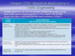
Chapter 7: Statistical Applications in Traffic Engineering. Chapter objectives: By the end of these chapters the student will be able to (We do skip simple descriptive stats because they were covered in CE361 and in an undergrad statistics class.):. 7.8 Hypothesis testing.

Chapter 7: Statistical Applications in Traffic Engineering
E N D
Presentation Transcript
Chapter 7: Statistical Applications in Traffic Engineering Chapter objectives: By the end of these chapters the student will be able to (We do skip simple descriptive stats because they were covered in CE361 and in an undergrad statistics class.):
7.8 Hypothesis testing Two distinct choices: Null hypothesis, H0 Alternative hypothesis: H1 E.g. Inspect 100,000 vehicles, of which 10,000 vehicles are “unsafe.” This is the fact given to us. H0: The vehicle being tested is “safe.” H1: The vehicle being tested is “unsafe.” In this inspection, 15% of the unsafe vehicles are determined to be safe Type II error (bad error) and 5% of the safe vehicles are determined to be unsafe Type I error (economically bad but safety-wise it is better than Type II error.)
Types of errors Steps of the Hypothesis Testing Decision Reality • State the hypothesis • Select the significance level • Compute sample statistics and estimate parameters • Compute the test statistic • Determine the acceptance and critical region of the test statistics • Reject or do not reject H0 Reject H0 Accept H0 H0 is true Type I error Correct Correct Type II error H1 is true Fail to reject a false null hypothesis: Accept a false H0 Reject a correct null hypothesis: Reject a true H0 P(type I error) = (level of significance) P(type II error ) =
Dependence between , , and sample size n There is a distinct relationship between the two probability values and and the sample size n for any hypothesis. The value of any one is found by using the test statistic and set values of the other two. • Given and n, determine . Usually the and n values are the most crucial, so they are established and the value is not controlled. • Given and , determine n. Set up the test statistic for and with H0 value and an H1 value of the parameter and two different n values. (Read the handout given in class carefully to understand this. Notice we need to compute d value to find these.) Here we are comparing means; hence divide σ by sqrt(n). The t (or z) statistics is: t or z
7.8.2 Before-and-after tests with generalized alternative hypothesis • The significance of the hypothesis test is indicated by , the type I error probability. = 0.05 is most common: there is a 5% level of significance, which means that on the average a type I error (reject a true H0) will occur 5 in 100 times that H0 and H1 are tested. In addition, there is a 95% confidence level that the result is correct. 0.025 each • If H1 involves a not-equal relation, no direction is given, so the significance area is equally divided between the two tails of the testing distribution. Two-sided • If it is known that the parameter can go in only one direction, a one-sided test is performed, so the significance area is in one tail of the distribution. 0.05 One-sided upper
Two-sided or one-sided test These tests are done to compare the effectiveness of an improvement to a highway or street by using mean speeds. • If you want to prove that the difference exists between the two data samples, you conduct a two-way test.(There is no change.) • If you are sure that there is no decrease or increase, you conduct a one-sided test. (There was no decrease) Null hypothesis H0: 1 = 2 (there is no change) Alternative H1: 1≠ 2 Null hypothesis H0: 1 = 2 (there is no increase) Alternative H1: 1 2
Example (p.137-138) The decision point (or typically zc: • For two-sided: 1.96*1.53 = 2.998 • For one-sided: • 1.65*1.53 =2.525 |µ1 - µ2| = |60-55| = 5 > zc By either test, H0 is rejected. At significance level = 0.05 (See Table 7-3.) You can compute z score and compare Z computed and Z critical values.
Use of the standard normal distribution table, Tab 7-3 Table 7-3 Z = 1.43 Most popular one is a 95% confidence level and both sided µ ± 1.96 . See section 7.2.2 for confidence interval. Excel functions: NORMSDIST(z) and NORMSINV(cum prob)
7.8.3 Other useful statistical tests The t-test (for small samples, n<=30) – Table 7.6: tc = 2.101 for two-sided α = 0.05. (See the samples in page 140)
F-test - Table 7.7 The F-Test to test if s1=s2 When the t-test and other similar means tests are conducted, there is an implicit assumption made that s1=s2. The F-test can test this hypothesis. The numerator variance > The denominator variance when you compute a F-value. If Fcomputed≥ Ftable(n1-1, n2-1, a), then s1≠s2 at a asignificance level. If Fcomputed < Ftable (n1-1, n2-1,a), then s1=s2 at a asignificance level. Discuss the problem in p.140.
Paired difference test You perform a paired difference test only when you have a control over the sequence of data collection. e.g. Simulation You control parameters. You have two different signal timing schemes. Only the timing parameters are changed. Use the same random number seeds. Then you can pair. If you cannot control random number seeds in simulation, you are not able to do a paired test. Table 7-8 shows an example showing the benefits of paired testing The only thing changed is the method to collect speed data. The same vehicle’s speed was measured by the two methods.
Paired or not-paired example (Table 7.8) H0: No increase in test scores (means one-sided or one-tailed) Tab 7.6 for t values Not paired: Paired: tcritical = 1.701 for df=28, a = 0.05. Computed 1.5807 < Critical t = 1.701 Hence, H0 is NOT rejected. tcritical = 1.761 for df=14, a = 0.05. Computed 11.218 < Critical t = 1.761. Hence, H0 is clearly rejected.
Chi-square (2-) goodness-of-fit test Example: Distribution of height data in Table 7-9. H0:The underlying distribution is uniform. H1: The underlying distribution is NOT uniform. The authors intentionally used the uniform distribution to make the computation simple. We will test a normal distribution in class using Excel.
Steps of Chi-square (2-) test • Define categories or ranges (or bins) and assign data to the categories and find ni = the number of observations in each category i. (At least 5 bins and each should have at least 5 observations.) • Compute the expected number of samples for each category (theoretical frequency), using the assumed distribution. Define fi = the number of samples for each category i. • Compute the quantity:
Steps of Chi-square (2-) test (cont) • 2 is chi-square distributed (see Table 7-11). If this value is low, our hypothesis is correct. Usually we use = 0.05 (5% significance level or 95% confidence level). When you look up the table, the degree of freedom is f = N – 1 – g where g is the number of parameters we use in the assumed distribution. For normal distribution g = 2 because we use µ and to describe the shape of normal distribution. (For the uniform distribution in the example g = 0. Hence, f = 10 – 1 – 0 = 9. • If the computed 2 value is smaller than the critical c2 value, we accept H0.
What’s the Chi-square (2-) test testing? You need to know how to pull out values from the assumed distribution to create the expected histogram. Assumed distribution Chi-square (2-) test Expected distribution (or histogram) Actual histogram