
Advanced Techniques in Lighting and Rendering Models
E N D
Presentation Transcript
Lighting • Rendering • Light source • Reflection models • Shading models
Rendering • Concerned with determining the most appropriate colour (i.e. RGB tuple) to assign to a pixel associated with an object in a scene • We need to know • how to describe light sources • how light interacts with materials - reflection models • how to calculate the intensity of light that we see at a given point on object surface - shading models
A Model for Lighting • Only light that reaches the viewers eye is ever seen • Direct light is seen as the colour of the light source • Indirect light depends on interaction properties • In computer graphics we replace viewer with projection plane • Rays which reach COP after passing through viewing plane are actually seen
Illumination Variables • Light source • Positions • Properties • Object • Geometry of the object at that point (normal direction) • Material properties • opaque/ transparent, shiny/dull, texture surface patterns • Position and orientation of view plane
Modelling the Light Source • Light sources characterized by the illumination function: • Contribution of a light source can be determined by integrating over the surface of the light source • For real-time speeds it is easier if we can approximate with point source (or set of point sources) • (x, y, z) : point on light source surface • (q, f) : direction of emission • : wavelength
Light sources • Ambient light – uniform lighting • Point source – emits light equally in all directions • Spotlight – characterized by a narrow range of angles through which light is emitted • Distance light sources – parallel rays of light
Reflection Model • A reflection model (also called lighting or illumination model) describes the interaction between light and a surface • The nature of interaction is determined by the material property • Three general types of interaction: specular reflection, diffuse reflection, transmission
Reflection Model • Ambient - reflected from other surfaces • Diffuse - from a point source reflected equally in all directions • Specular - from a point source reflected in a mirror-like fashion specularity
The Phong Reflection Model • The Phong Illumination Model is a local illumination model and is largely an empirical model. However it is fast to compute and gives reasonably realistic results. • Light incident upon a surface may be reflected from a surface in two ways: • Diffuse reflection: Light incident on the surface is reflected equally in all directions and is attenuated by an amount dependent upon the physical properties of the surface. Since light is reflected equally in all directions the perceived illumination of the surface is not dependent on the position of the observer. Diffuse reflection models the light reflecting properties of matt surfaces. • Specular Reflection: Light is reflected mainly in the direction of the reflected ray and is attenuated by an amount dependent upon the physical properties of the surface. Since the light reflected from the surface is mainly in the direction of the reflected ray the position of the observer determines the perceived illumination of the surface. Specular reflection models the light reflecting properties of shiny or mirror-like surfaces.
The Phong Reflection Model • A local illumination model including only contributions from diffuse and specular components suffers from one large drawback, namely, a surface that does not have light incident on it will reflect no light and will therefore appear black. • This is not realistic, for example a sphere with a light source above it will have its lower half not illuminated. In practice in a real scene this lower half would be partially illuminated by light that had been reflected from other objects. This effect is approximated in a local illumination model by adding a term to approximate this general light which is `bouncing' around the scene. This term is called the ambient reflection term and is modelled by a constant term. Again the amount of ambient light reflected is dependent on the properties of the surface. • Hence the local illumination model that is generally used is illumination = Ambient + Diffuse + Specular
surface P Ambient Reflection In the Phong model ambient light is assumed to have a constant intensity throughout the scene. Each surface, depending on its physical properties, has a coefficient of ambient reflection which measures what fraction of this light is reflected from the surface. Hence for an individual surface the intensity of ambient light reflected is: I = Ka La I = Reflected intensity Ka = Reflection coefficient Ia = Ambient light intensity (same at every point)
Diffuse Reflection A perfectly diffuse reflecting surface scatters light equally in all directions. Thus the intensity at a point on a surface as perceived by the viewer does not depend on the position of the viewer. The colour of the light reflected from the surface depends upon the colour of the light and the properties of the surface. Light incident on the surface will have some components absorbed and others scattered thus giving the surface its colour. Thus a surface that appears red under white light absorbs green and blue and scatters red light. When only diffuse light is considered surfaces will appear dull or matt.
light source light source N R eye L V surface P Diffuse Reflection The intensity due to diffuse reflection is given by Lambert's cosine law: Id= Kd Ii cos Id = Reflected intensity Kd = Diffuse reflection coefficient Ii = Intensity of the incident light If there is more than one light source then the diffuse intensity is summed over all light sources.
The Effect of Distance With the lighting model proposed so far two surfaces with the same properties and orientation but different distances from the light source would have the same intensity of illumination. This can be corrected by including a factor dependent on the distance of the surface point to the viewing point. Hence the lighting model (for a single light source) and modelling only ambient and diffuse reflection is now: where r is the distance and k is an arbitrary constant chosen to make the image appear correct.
Specular Reflection • Specular reflection is caused by the mirror-like properties of a surface. A perfect mirror will reflect light arriving at the surface at an angle of incidence theta to the normal at a reflected angle of theta to the normal in the same plane as the normal and the incident light. This means that only a viewer on the reflected ray will actually see the reflected light. light source N R eye L surface
light source N R eye L V surface Specular Reflection • In practice no surface is a perfect mirror and there will be a certain amount of light scattered around the reflected direction. • The reflected light is therefore seen over an area of the surface as a highlight. The colour of this specularly reflected highlight is usually taken to be that of the light source. In diffuse reflection the reflected light is the colour of the surface. • In practice the distribution function for specularly reflected light is a complex function of Phi - the angle between the reflected ray and the viewing direction V.
light source N R eye L V surface Specular Reflection • Amount of light visible to viewer depends on the angle between R and V: • Is = KsIi(cos)n • n varies with material, large n: shiny, small n: dull V = Direction to the viewer (COP) R = Direction of perfect reflected light N = Surface normal L = Direction of light source Ii = Intensity of the incident light Ks = Specular reflection coefficient Is = Reflected intensity
light source light source Specular Reflection N • In perfect specular reflection, light is reflected along the direction symmetric to the incoming light • In practice, light is reflected within a small angle of the perfect reflection direction - the intensity of the reflection tails off at the outside of the cone. This gives a narrow highlight for shiny surfaces, and a broad highlight for dull surfaces R P N R P
I n=1 n=10 Specular Reflection • Thus we want to model intensity, I, as a function of angle between viewing direction and the reflection, say , with a sharper peak for shinier surfaces, and broader peak for dull surfaces • This effect can be modelled by (cos)n, with a sharper peak for larger n • Empirical
n = 5 n = 15 n = 1005 n = 45 Specular Highlights • The cosine function (defined on the sphere) gives us a lobe shape which approximates the distribution of energy about a reflected direction controlled by the shinyness parameter a known as the Phong exponent. (cos)n
light source N R eye L V surface Ambient, Diffuse and Specular Hence we obtain the complete basic reflection model: Note that it is assumed that N, R and V are unit vectors The coefficient of Specular Reflection is treated as a constant in the Phong model. However it is actually a function of the angle of incidence.
Colour • To handle colour the usual approach is to treat specular highlights as being the same colour as the light source. • The colour of objects is handled by treating the coefficients of ambient and diffuse reflection as having red, green and blue components. Hence the red, green and blue signals that drive the display are produced from: The Diffuse and Specular terms are summed over each light source
Summary of the Phong Model • Light sources are usually considered as point sources situated infinitely far away. Hence the angle between the incident light and the normal to a planar surface is constant over a planar surface. • The viewer is assumed positioned at infinity, hence the angle between the viewing direction and the reflected ray is constant over a planar surface. • The diffuse and specular terms are modelled as local components only. • An empirical result is used to model the distribution of the specular term around the reflection vector. • The colour of the specular term is assumed to be that of the light source. • The global illumination is modelled as a constant ambient term. • Shadows are not handled. • The coefficient of diffuse reflection is wavelength dependent. But it is sampled at each of the three primary colours. • The coefficient of specular reflection is modelled as a constant but is actually dependent on the angle of incidence.
Local Shading Models • Local shading models provide a way to determine the intensity and color of a point on a surface • They do not require knowledge of the entire scene, only the current piece of surface. • For the moment, assume: • We are applying these computations at a particular point on a surface • We have a normal vector for that point
Flat Shading • Compute shading at a representative point and then generalise to the whole polygon • For a flat polygon the vector n is constant across the surface • If we assume a distant viewer, v is constant • If we assume a distant light source l is constant • If the three vectors are constant then the shading calculation needs to be calculated only once for each polygon
Flat Shading • Calculate normal • Assume L.N and R.V constant (light & viewer at infinity) • Calculate Ir, Ig, Ib using Phong reflection model • Project vertices to viewplane • Use scan line conversion to fill polygon light viewer N V L R
Flat Shading • When flat shading is used the same shade is used over the whole surface. If the surface actually corresponds to a planar surface in the model then this is correct. Though remember that as the Phong Illumination Model assumes that the light source is at infinity a large surface illuminated by a light positioned close to the surface will not be evenly illuminated in reality. • The shade to be associated with a surface is calculated before View Transformation and Perspective Transformation are carried out. That is before all the angles are distorted. • If flat shading of a planar surface is to be considered then an arbitrary point on the surface can be chosen at which to calculate the shade. • If a curved surface is approximated by a mesh of polygonal facets then two approaches to calculating the shade of the facets can be used: • Calculate the shade at some point on each facet, for example its centre. • Calculate the shade at the vertices of the mesh using true surface normals. The shade at each facet can then be evaluated as the average of the shades at its vertices. • Flat shading provides realistic images of objects which are composed entirely of planar surfaces but produce a facetted appearance when used to approximate curved surfaces.
2D Graphics - Filling a Polygon • Scan line methods used to fill 2D polygons with a constant colour • find ymin, ymax of vertices • from ymin to ymax do: • find intersection with polygon edges • fill in pixels between intersections using specified colour
Smooth Shading • In many cases the polygons that are to be rendered in the polygon pipeline are an approximation to a curved surface. • In this case the different shade calculated on each planar polygon will give a facetted appearance to the surface and it will not look like a smooth curved surface at all. • To avoid this problem incremental, or smooth, shading methods are used to produce smoothly shaded pictures from planar polygon facetted representations of curved surfaces.
Smooth Shading • The first step is to produce a shade value at each vertex of the polygonal mesh representing the surface. This can be done in two ways: • Evaluate a surface normal on each polygonal facet. Produce a surface normal at each vertex by averaging the surface normals for the surrounding facets. The shade at the vertex can now be calculated. • Evaluate the shade directly at each vertex by considering the vertex as a point on the actual curved surface and evaluating the actual surface normal to the surface at that point. • Once the shade at the vertices of the polygonal mesh are known the shade at points interior to the polygonal facets are interpolated from the values at the vertices. • This technique makes curved surfaces look `smooth shaded' even though based on a planar facet representation. The interpolation of shade values is incorporated into the polygon scan conversion routine. • Hence an increase in realism is obtained at far less expense in computation than carrying out a pixel-by-pixel shading calculation over the whole original surface.
Gouraud Shading • Gouraud shading is a method for linearly interpolating a colour or shade across a polygon. It was invented by Gouraud in 1971 • It is a very simple and effective method of adding a curved feel to a polygon that would otherwise appear flat • It can also be used to depth queue a scene, giving the appearance of objects in the distance becoming obscured by mist Henri Gouraud is another pioneering figure in computer graphics
N Gouraud Shading • Gouraud shading attempts to smooth out the shading across the polygons • Unlike a flat shaded polygon, it specifies a different shade for each vertex of a polygon • The rendering engine then smoothly interpolates the shade across the surface
Gouraud Shading • Begin by calculating the normal at each vertex • A feasible way to do this is by averaging the normals from surrounding polygons • Then apply the reflection model to calculate intensities at each vertex
P3 P3 P2 P2 1- Q Q P P P1 P1 P4 Gouraud Shading • We use linear interpolation to calculate intensity at edge intersection P IPRED = (1-)IP1RED + IP2RED where P divides P1P2 in the ratio 1- • Similarly for Q • Then we do further linear interpolation to calculate colour of pixels on scanline PQ
Gouraud Shading • Bilinear interpolation:
Gouraud Shading Limitations • Constant shading is simple, but it emphasizes the polygonal nature of the model. Our perceptual system exaggerates the effect because we see very clearly the boundary between adjacent light and dark shades (Mach banding) • Problems with Gouraud shading occur when you work with large polygons. A specular highlight at a vertex tends to be smoothed out over a larger area than it should cover - imagine you have a large polygon, lit by a light near it's center. The light intensity at each vertex will be quite low, because they are far from the light. The polygon will be rendered quite dark, but this is wrong, because it's centre should be brightly lit • Gouraud shading can make a real difference over flat shaded polygons
Gouraud Limitations - Mach Bands • The rate of change of pixel intensity is even across any polygon, but changes as boundaries are crossed • This ‘discontinuity’ is accentuated by the human visual system, so that we see either light or dark lines at the polygon edges - known as Mach banding • Mach bands where the intensity is constant in bands – similar effect with Gouraud shading
Phong Shading • Phong shading uses similar principles to Gouraud shading but instead of interpolating the shade across the surface it is the surface normals that are interpolated. The interpolated normals are then used to evaluate a shade at each pixel. • As before the light source and the viewer are assumed to be at infinity so that the intensity at a point is a function only of the interpolated normal. • The equations for the interpolated normals are similar to Gouraud shading but each component of the normal has to be interpolated and the vector re-normalised after each interpolation step.
P3 P3 P2 P2 N2 N2 N N Q Q P P N1 N1 P1 P1 P4 P4 Phong Shading • Phong shading interpolates normals at each pixel, then apply the reflection model at each pixel to calculate the intensity IRED, IGREEN, IBLUE (shade each pixel individually) • Every single pixel has it's brightness calculated using the interpolated normal vector
Phong Shading • For a pixel on this polygon, the fraction of light from the light source reflecting off this pixel is the dot product of n and I. • The dot product function returns values in the range 1 to -1. 1 is full brightness. • There is no such thing as negative light, so values less then 0 should be taken as 0. • If you multiply this value by the brightness of the light, then you have the brightness of that pixel
Phong versus Gouraud Shading • A major advantage of Phong shading over Gouraud is that specular highlights tend to be much more accurate, vertex highlight is much sharper • The cost is a substantial increase in processing time because reflection model applied per pixel • But there are limitations to both Gouraud and Phong • In practice, some simplifications are made to the model for efficiency. For example, ambient light is sometimes assumed to be a constant
Shading Summary • It is expensive to calculate the intensity at each pixel of a projected polygon, and so there is a family of methods which use interpolation to calculate intermediate values • constant shading: reflection calculation is carried out once for each polygon, and the polygon is assigned a constant shade according to that calculation • Gouraud shading: an estimate is made of the normal at each vertex of a polygon (for example, by averaging the normals of all surrounding polygons); reflected intensity at each vertex is then calculated; linear interpolation is then used to estimate the intensity at any interior pixel as the shading is carried out • Phong shading: as with Gouraud, normal estimates are made at each vertex; but in contrast, we proceed to interpolate the normals at each pixel and then calculate the intensity for that pixel