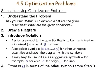

Flexible Optimization Problems
E N D
Presentation Transcript
Flexible Optimization Problems A. Akavia, S. Safra
Motivation What do we do with all the NP-Complete problems ???
Relaxations: 2 Parameters • Optimization function approximation • Input flexibility Example – graph coloring problem: • Optimization function – • find an approximation of the min coloring. • Input flexibility – • find a k-coloring with few monochromatic edges.
Talk Plan • Approximation • Input flexibility • Flexible optimization problems • Natural examples • Definitions • Hardness results
Relaxation 1: Approximation • An approximation algorithm is an algorithm that returns an answer C which is “g-approximate” to the optimal solution C*. • C g C*(minimization) • 1/g C* C(maximization)
Relaxation 2: Input Flexibility • Graph Editing problems • Max instances satisfaction problems • Property Testing
Input FlexibilityGraph Editing problems Input: • a graph G, and • a desired property Goal: finding a small set of edge modifications (addition/deletion/both) that transform the graph Ginto a graph G’with the desired property.
Input FlexibilityGraph Editing problems • Examples: • Chain graph • Perfect graph • Applications: • computational biology • numerical algebra • Known complexity and approximation results are w/r to the number of modifications
Input FlexibilityMax instances satisfaction problems • Given a set of instances, satisfy as many as possible: • Max SAT • Max k-colorable subgraph
Input FlexibilityProperty Testing • Distinguish, by only a very small number of probes, between instances x that • satisfy a given property accept • no set of |x| modifications causes x to satisfy the property reject
Approximation of Flexible Optimization Problems • Combining both relaxations – approximation and input flexibility.
Examples of Natural Flexible Optimization Problems • Min Synthesis Graph • Min Non-Deterministic Automaton • Min Hidden Markov Model
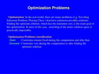
* * * * * * * * * * * * * * * * * * * * * * * * * * * * * * * * * * * * * * * * * * * * * * * * * * * * * * * * * * * * * * * * * * * * * * * * * * * * * * * * * * * * * * * * * * * * * * * * * * * * * * * * * * * * * * * * * * * * * * * * * * * * * * * * * * * * * * * * * * * * * * * * * * * * * * * * * * * * * * * * * * * * * * * * * * * * * * * * * * * * * * * * * * * * * * * * * * * * * * * * * * * * * * * * * * * * * * * * * * * * * * * * * * * * * * * * * * * * * * * * * * * * * * * * * * * * * * * * * * * * * * * * * * * * * * * * * * * * * * * * * * * * * * * * * * * * * * * * * * * * * * * * * * * * * * * * * * * * * * * * * * * * * * * * * * * * * Combinatorial Chemistry Synthesizing and screening sets of compounds, which best represent the relevant property space greatly enhance the success of lead identification and optimization Property space – a multi dimensional space molecular property coordinate molecule point similarity (molecules) distance (points) Lead optimization Lead identification Focused library diverse library *
associated set of beads Synthesis Processes - Multi Route Mix & Split a b c b a b c a a b c b a b c a Node - grow step Label - appended unit a b b c c a b c b a b a b a b c a a b b b b b b c c a b c b a b a b a b c a a b b b b b b c c a b a a a b b c c c c b a b a b a b a b c a Schematic representation a b b b b b b b b c c a a a b b b b c c c c
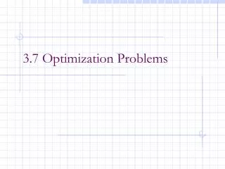
Input flexibitily– • producing more strings • Approximation – • finding a small synthesis graph • not the minimum a b c Flexible Min Synthesis Graph a b c a b c a b Input: • S - a set of n strings of length L, • d- a bound on the number of excess strings Goal: Find a synthesis graph G • that produces all strings in S and • no more than d extra strings. (Input Flexibility) • with minimum number of internal nodes(Optimization)
Non-Deterministic Finite Automaton (NFA) • Many applications: • program verification • language and speech recognition • Natural language processing and natural linguistics • control design Prop.: Finding a minimum NFA that accepts a given language L is hard. Proof: Just deciding whether an NFA accepts all strings is PSPACE-hard.
Flexible Min NFA • It would suffice, for many applications, to construct an automaton that accepts a language “similar” to the input one.(Input Flexibility) • Many applications could benefit greatly from being able to efficiently find a small NFA accepting a given language L.(Optimization)
Example: Automata-Theoretic Approach to Program Verification • ProgramP is correct with respect to a specificationsT if: L(P) L(T)(regard P as an automaton of all program computations) • In concurrent programming: processesP1,..., Pn are correct w/r to specificationT if: L(P1) ... L(Pn) L(T) • L(P1) ... L(Pn) = L(P), where P=P1x…x Pn in the worst case, |P| is exponential in n
Example: Automata-Theoretic Approach to Program Verification • Coping with this state-explosion: • finding a small automaton P’ (Optimization) • such that L(P) L(P’)(Input Flexibility) • and then checking whether L(P') L(T)
Flexible Min Hidden Markov Model Input: a training sample set Output: a Hidden Markov Model • reasonable size(Optimization) • generates a probability distribution similar to the one from which the training data was drawn (Input Flexibility) • Many applications: • speech recognition • bioinformatics - gene finding, sequence alignment and protein modeling • handwriting and visual recognition.
General Notion of Flexibility Not necessarily a metric • Def: assume a distance function(x,x’)to be the smallest number of basic modifications (say, bit-changes) necessary in order to transform x to x’. the ball of radius d around a given input x is ball(x,d) = {x’ | (x,x’)d}
(d,g)-flexible approximation problem • A (d,g)-flexible approximation problem is a pair <,f> such that: • is a distance function between instances, • f is the maximization (minimization) function, • For any instance x and threshold t: • y f(x, y) taccept • x'ball(x,d) , y : f(x’, y) < t/greject • Otherwise “don't care”(either accept or reject) • In minimization: • f(x,y) taccept • f(x’,y) > gtreject • Otherwise “don't care”
Biclique Edge Cover - Definition Input: Bipartite graphG=(P,Q,E) Goal: Cover all edges by bicliques (i.e. complete bipartite subgraphs)
G’ (d,g)-Flexible Approximation Biclique Edge Cover • A (d,g)-flexible approximation Biclique Edge Cover is a pair<,f> such that: • (G,G’) is a the number of edges whose addition to Ggives G’ . • f(G,y) is the number of bicliques in the cover y. G f(G’,y)=2 f(G,y)=3 (G,G’)=4
Hardness of (d,g)-Flexible Approximation Biclique Edge Cover Thm: >0(d,g)-Flexible Approximation Biclique Edge Cover problem is hard for any g=O(|V|1/5-) and d=O(g), unless NP=ZPP. Proof: later.
a b c Synthesis Graph a b c a b c a b Input: • S - a set of n strings of length L, • d- a bound on the number of excess strings Goal: Find a synthesis graph G • that produces all strings in S and • no more than d extra strings. (Input Flexibility) • with minimum number of internal nodes(Optimization)
a b c (d,g)-Flexible Approximation Synthesis Graph a b c a b c a b A (d,g)-flexible approximation Synthesis Graph is a pair <,f> such that: • (S,S’) is a the number of strings whose addition to Sgives S’. • f(S,H) is the number of internal nodes in a synthesis graph H that produces the strings S.
Hardness of (d,g)-Flexible Approximation Synthesis Graph Thm: >0 (d,g)-Flexible Approximation Synthesis Graph problem is hard for any g=O(|S|1/10-) and d=O(g), unless NP=ZPP, even in the restricted case in which all words in S are of length 3, and all have the same second character. Proof:
Reduction Outlines • Reduction from Biclique Edge Cover: a b c a b c a b c { pAq| (p,q)E} a b Bipartite graph G Synthesis graph H Strings set S
A Define S = { pAq| (p,q)E} Define S A A Proof: Hardness with no flexibility Reduction from Biclique Edge Cover [CS]: k-biclique edge coverof G synthesis graph H with k internal nodes producing S H - a graph constructing S G=(P,Q,E) a bipartite graph.
A Define S = { pAq| (p,q)E} Define S A A Proof: Allowing flexibility Reduction from flexible approximation Biclique Edge Cover: k-biclique edge coverof G’in d-distance from G synthesis graph H with k internal nodes producing S’ in d-distance from S (d,g)-Flexible Approximation Synthesis Graph is hard for g=O(|S|1/10-) and d=O(g) G=(P,Q,E) a bipartite graph. H - a graph constructing S
(d,g)-Flexible Approximation Non-Deterministic Finite Automaton (NFA) • A (d,g)-flexible approximation NFA is a pair <,f> such that: • (L,L’) is a the number of words whose addition to Lgives L’ • f(L,A) is the number of states in the NFA A accepting L.
Hardness of (d,g)-Flexible Approximation NFA Thm: >0 (d,g)-Flexible Approximation NFA problem is hard for any g=O(|V|1/10-) and d=O(g), unless NP=ZPP, even in the restricted case in which all the words in L are of length 2.
v5 v4 v3 v2 v1 Define L Define L = { vu| (v,u)E} u5 u4 u3 u2 u1 qF q0 A - an automaton acceptin L Proof: Hardness with no flexibility Reduction from Biclique Edge Cover: k-biclique edge cover of G NFA with k+2 states,accepting L G=(P,Q,E) a bipartite graph.
Appendix Hardness Proof of(d,g)-Flexible Approximation Biclique Edge Cover
(d,g)-Flexible Approximation Biclique Edge Cover • A (d,g)-flexible approximation Biclique Edge Cover is a pair<,f> such that: • (G,G’) is a the number of edges whose addition to Ggives G’ . • f(G,y) is the number of bicliques in the cover y. G f(G,y)=3
Hardness of (d,g)-Flexible Approximation Biclique Edge Cover Thm: (d,g)-flexible approximation Graph-Coloring problem is hard for any g=O(|V|1/5-) and d=O(g), unless NP=ZPP. Proof: • (G) = min no. of bicliques in biclique edge cover • d(G) = min no. of bicliques in d-flexible biclique edge cover (i.e.d additional edges) Lemma: d(G)(G) d(G) + d
t t Hardness of (0,g)-Flexible Approximation Biclique Edge Cover Proof: First, establishing hardness in case d=0: [Simon] GBC- Biclique Edge Cover GC - Clique Cover sbiclique-cover in GBC(s – 2|EC|t)/t2clique-cover in GC rclique-cover in GC(t2 r + 2|EC| t)biclique-cover in GBC
t t Calculating Approximation Factor yC= (yBC- 2|EC|t) / t2 (gyBC* - 2|EC|t) / t2 = [g(t2 y*C + 2|EC|t) - 2|EC|t] / t2 = gyC* + (2|EC|/t) (g-1) 2gyC (t = 2|EC|) 2 c|VBC|xyC* (g = O(|VBC|x)) c (t2 |VC|)xyC* (|VBC| = t2 |VC|) = 4c (|EC|2|VC|)xyC*(t = 2|EC|) 4c (|VC|)5xyC*(|EC| |VC|5) Clique-Cover is hard to approx within O(|VC|1-), >0 [FK] BC is hard x s.t. (|VC|)5x |VC|1- (i.e. for x 1/5 - ) Hence BC is hard to approx in g=O(|VBC|1/5-), >0.
t t Hardness of (d,g)-Flexible Approximation Biclique Edge Cover Second, establishing hardness in case d=O(|V|1/5 - ): Same reduction as in case d=0: [Simon] GBC- Biclique Edge Cover GC - Clique Cover
Calculating Approximation Factor Claim: a solution yd whichg-approximate(d,g)-flexible Biclique Edge Cover problem, with g=O(|VBC|x) and d=O(g),gives a solution y whichg-approximateBiclique Edge Coverproblem. Proof: add a new biclique for each added edge. y 2|VBC|x (G) y = yd + d = gd(G) + d g(G) + d (since d(G)(G) d(G) + d) 2g(G) (since d = O(g)) = 2|VBC|x (G) Biclique Edge Cover is hard for g=O(|VBC|1/5-) (d,g)-flexible Biclique Edge Cover is hard for g=O(|VBC|1/5-) and d=O(g)
(d,g)-Flexible Approximation Graph Coloring • A (d,g)-Flexible Approximation Graph Coloring is a pair<,f> s.t. • (G,G’) is a the number of edges whose deletion from Ggives G’ • f(G,y) is the number of colors in the coloring y.
Hardness of (d,g)-Flexible Approximation Graph Coloring Thm: (d,g)-flexible approximation graph coloring problem is hard for any g=O(|V|1-) and d=O(g), unless NP=ZPP Proof: denote • (G) = min no. of colors to color G • d(G) =min no. of colors in d-flexible coloring (i.e. d monochromatic edges) Lemma: d(G)(G) d(G) + d
Hardness Proof Cont. If we had an approximation algorithm… • Let yd be a solution to (d,g)-flexible approximation Graph-Coloring problem • Note: d(G) |yd| gd(G) • By the lemma we may obtain a solution y to Graph-Coloring problem with|y| = |yd| + d gd(G) + d g(G) + d = O(g) (G) • But…It is hard to approximate Graph-Coloring problem by factor g, for any g = O(|V|1-) [FK]
Future Work • Parameterized polynomial solution to these problems • Approximation algorithm • Extending our results to other problems