Download
1 / 13
130 likes | 147 Views
This study examines the speed-dependent phase lag of solar wind Helium abundance across two solar cycles, revealing insights into Helium filtration processes and its impact on solar activity dynamics.

E N D
Helium Variation Across Two Solar Cycles Reveals A Speed-Dependent Phase Lag B. L. Alterman & Justin C. Kasper July 18, 2019
Solar Wind Helium Abundance &Sunspot Number (SSN) Definitions Published Observations Strongest in slow wind ( Falls off for Helium vanishing speed Within 1 of min observed Possibly indicates helium essential to solar wind formation • Hydrogen (Protons) • 95 % by number density • Fully Ionized Helium (Alphas) • 4% by number density • Helium Abundance • & SSN Cross Correlation
Data Sources Solar Wind Ions SSN 13 month smoothed SSN Solar Information Data Center (SIDC) • Wind/SWE FCs • Solar cycles 23 & 24; end of cycle 22 • > 23 years • Covers one Hale cycle • Long-term stability of SWE/FC system essential to this study
& SSN • Trailing end of cycle 22 through decline of cycle 24. • SSN in black, dashed • colored lines. • 10 quantiles • Color & symbol • Covers 312 km/s to 574 km/s • Take 250 day averages of all data • Legend
& SSN • Present drop in indicates entering minimum 25 • peaks at • Meaningful () up to • Highly significant () up to • Phase offset between and SSN • returns to same value at Max 23 & 24, even though different cycle amplitudes
Time-Lagged Cross Correlation • Calculate for delay times -200 days to 600 days, steps of 40 days • Delay time is time for which peaks as function of delay. • Plot Observed (open) and Delayed (filled) • Error bars are repeat of procedure for 225 to 275 day averages
Time-Lagged Cross Correlation • Delayed for all • Observed & Delayed peak at • Largest in fast wind • Most significant in slow wind
Phase Delay: • (Top) Observed • Hysteresis present • Time is counter clock (color bar) • (Bottom) Delayed • Larger indicates spread of about trend decreases • indicates linear model better in Delayed case • As expected, fit parameters are identical.
Delay of Peak • Positive delay = SSN precedes • Speed of instantaneous response OR • Two delays • Either case, time lag is present
Robustness • Helium vanishing speed • Kasper+ (2007), black dashed • Low solar activity across Hale cycle • Suitable for comparison to Kasper+ (2007)
Robustness • All SSN (Unfilled) • selects solar activity conditions similar to Min 25 • Consistent in both cases • Better agreement for • Discrepancy for expected
Helium Filtration • Phase offset w/rt SSN observed in many solar indices • Lyman-alpha • Measures chromosphere & transition region activity • 125 day • Soft x-ray flux (SXR) • Measures active regions (ARs) • > 300 day • Speed-dependent phase lag suggests processes above the photosphere modify
Helium Filtration • Two slow wind sources • Streamer belt • Weak B • Magnetically closed • Long-lived loops • ARs • Strong B • Higher latitudes than Streamer Belt • More open flux • If two delays • is streamer belt • is ARs • reflects extent B is open • FIP effect • First Ionization Potential (FIP) • Ion abundances differ from photospheric value • Low FIP (< 10 eV) increase • High FIP show apparent depletion • Strongest in upper chromosphere & transition region • Weakens with B • Increases with loop length and age • Gravitational settling • interchange reconnection • Not mutually exclusive