Particle Physics
280 likes | 296 Views
Learn how to calculate cross sections using Quantum Electrodynamics (QED) in electron-positron annihilation. Includes Feynman diagrams, matrix elements, and spin calculations.

Particle Physics
E N D
Presentation Transcript
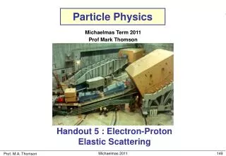
Particle Physics Michaelmas Term 2011 Prof Mark Thomson Handout 4 : Electron-Positron Annihilation Michaelmas 2011
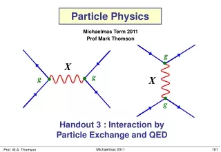
m+ e+ g m– e– g m+ m+ e+ e+ g m– e– e– m– QED Calculations How to calculate a cross section using QED (e.g. e+e– m+m–): Draw all possible Feynman Diagrams • For e+e– m+m– there is just one lowest order diagram + many second order diagrams + … + +… For each diagram calculate the matrix element using Feynman rules derived in handout 4. Sum the individual matrix elements (i.e. sum the amplitudes) • Note: summing amplitudes therefore different diagrams for the same final • state can interfere either positively or negatively! Michaelmas 2011
For QED the lowest order diagram dominates and • for most purposes it is sufficient to neglect higher order diagrams. m+ e+ g m– e– g m+ e+ m– e– and then square this gives the full perturbation expansion in Calculate decay rate/cross section using formulae from handout 1. • e.g. for a decay • For scattering in the centre-of-mass frame (1) • For scattering in lab. frame (neglecting mass of scattered particle) Michaelmas 2011
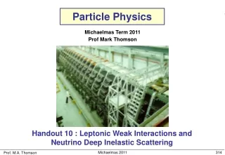
m– e– e+ m+ m+ e+ g • Incoming anti-particle • Incoming particle • Adjoint spinor written first m– NOTE: e– Electron Positron Annihilation e+e– m+m– • Consider the process: • Work in C.o.M. frame (this is appropriate • for most e+e–colliders). • Only consider the lowest order Feynman diagram: • Feynman rules give: • In the C.o.M. frame have with Michaelmas 2011
Electron and Muon Currents • Here and matrix element • In handout 2 introduced the four-vector current which has same form as the two terms in [ ] in the matrix element • The matrix element can be written in terms of the electron and muon currents and • Matrix element is a four-vector scalar product – confirming it is Lorentz Invariant Michaelmas 2011
e– e+ e+ e– e+ e– e+ e– RL RR LL LR Spin in e+e– Annihilation • In general the electron and positron will not be polarized, i.e. there will be equal • numbers of positive and negative helicity states • There are four possible combinations of spins in the initial state ! • Similarly there are four possible helicity combinations in the final state • In total there are 16 combinations e.g. RLRR, RLRL, …. • To account for these states we need to sum over all16 possible helicity • combinations and then average over the number of initial helicity states: • i.e. need to evaluate: for all 16 helicity combinations ! • Fortunately, in the limit only 4 helicity combinations give non-zero matrix elements – we will see that this is an important feature of QED/QCD Michaelmas 2011
In the C.o.M. frame in the limit m– e– e+ m+ • Left- and right-handed helicity spinors (handout 3) for particles/anti-particles are: where and • In the limit these become: • The initial-state electron can either be in a left- or right-handed helicity state Michaelmas 2011
m– m+ m– m+ • first consider the muon current for 4 possible helicity combinations m– m– m– RL LR LL RR m+ m+ m+ • For the initial state positron can have either: • Similarly for the final state m–which has polar angle and choosing • And for the final state m+ replacing obtain using • Wish to calculate the matrix element Michaelmas 2011
Consider the combination using The Muon Current • Want to evaluate for all four helicity combinations • For arbitrary spinors with it is straightforward to show that the • components of are (3) (4) (5) (6) with Michaelmas 2011
m– m+ m– m+ m– m+ m– • IN THE LIMIT only two helicity combinations are non-zero ! m+ • Hence the four-vector muon current for the RL combination is • The results for the 4 helicity combinations (obtained in the same manner) are: RL RR LL LR • This is an important feature of QED. It applies equally to QCD. • In the Weak interaction only one helicity combination contributes. • The origin of this will be discussed in the last part of this lecture • But as a consequence of the 16 possible helicity combinations only • four given non-zero matrix elements Michaelmas 2011
m– m– e– e– MRL e+ e+ MRR m– m+ m+ m+ m– m– MLR MLL e– e– e+ e+ m+ m+ m– m+ Electron Positron Annihilation cont. e+e– m+m– • For now only have to consider the 4 matrix elements: • Previously we derived the muon currents for the allowed helicities: • Now need to consider the electron current Michaelmas 2011
Taking the Hermitian conjugate of the muon current gives The Electron Current • The incoming electron and positron spinors (L and R helicities) are: • The electron current can either be obtained from equations (3)-(6) as before or • it can be obtained directly from the expressions for the muon current. Michaelmas 2011
e– e+ e– e+ • Taking the complex conjugate of the muon currents for the two non-zero • helicity configurations: To obtain the electron currents we simply need to set Michaelmas 2011
m– e– e+ m+ Matrix Element Calculation • We can now calculate for the four possible helicity combinations. e.g. the matrix element for which will denote Here the first subscript refers to the helicity of the e-and the second to the helicity of the m-. Don’t need to specify other helicities due to “helicity conservation”,only certain chiral combinations are non-zero. • Using: gives where Michaelmas 2011
MRR MRL MLR MLL m– m– m– m– e– e– e– e– e+ e+ e+ e+ m+ m+ m+ m+ cosq cosq cosq cosq -1 -1 -1 -1 +1 +1 +1 +1 Similarly • Assuming that the incoming electrons and positrons are unpolarized, all 4 • possible initial helicity states are equally likely. Michaelmas 2011
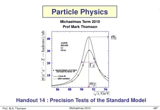
Mark II Expt., M.E.Levi et al., Phys Rev Lett 51 (1983) 1941 -1 +1 cosq Differential Cross Section • The cross section is obtained by averaging over the initial spin states • and summing over the final spin states: Example: e+e– m+m– pure QED, O(a3) QED plus Z contribution Angular distribution becomes slightly asymmetric in higher order QED or when Z contribution is included Michaelmas 2011
The total cross section is obtained by integrating over using giving the QED total cross-section for the process e+e– m+m– • Lowest order cross section calculation provides a good description of the data ! This is an impressive result. From first principles we have arrived at an expression for the electron-positron annihilation cross section which is good to 1% Michaelmas 2011
m– e– e+ • Similarly the muon and anti-muon are produced in a total spin 1 state aligned • along an axis with polar angle m+ • Hence where corresponds to the spin state, , of • the muon pair. • To evaluate this need to express in terms of eigenstates of Spin Considerations • The angular dependence of the QED electron-positron matrix elements can be understood in terms of angular momentum • Because of the allowed helicity states, the electron and positron interact • in a spin state with , i.e. in a total spin 1 state aligned along the • z axis: or e.g. MRR • In the appendix (and also in IB QM) it is shown that: Michaelmas 2011
Using the wave-function for a spin 1 state along an axis at angle m– e– MRR e+ m+ cosq cosq -1 -1 +1 +1 can immediately understand the angular dependence m– MLR e– e+ m+ Michaelmas 2011
m– e– e+ m+ Lorentz Invariant form of Matrix Element • Before concluding this discussion, note that the spin-averaged Matrix Element • derived above is written in terms of the muon angle in the C.o.M. frame. • The matrix element is Lorentz Invariant (scalar product of 4-vector currents) • and it is desirable to write it in a frame-independent form, i.e. express in terms • of Lorentz Invariant 4-vector scalar products • In the C.o.M. giving: • Hence we can write • Valid in any frame ! Michaelmas 2011
The helicity eigenstates for a particle/anti-particle for are: CHIRALITY where • Define the matrix • In the limit the helicity states are also eigenstates of • In general, define the eigenstates of as LEFT and RIGHT HANDED CHIRAL states i.e. • In the LIMIT (and ONLY IN THIS LIMIT): Michaelmas 2011
This is a subtle but important point: in general the HELICITY and CHIRAL eigenstates are not the same. It is only in the ultra-relativistic limit that the chiral eigenstates correspond to the helicity eigenstates. • Chirality is an import concept in the structure of QED, and any interaction of the form • In general, the eigenstates of the chirality operator are: • Define the projection operators: • The projection operators, project out the chiral eigenstates • Note projects out right-handed particle states and left-handed anti-particle states • We can then write any spinor in terms of it left and right-handed • chiral components: Michaelmas 2011
Chirality in QED • In QED the basic interaction between a fermion and photon is: • Can decompose the spinors in terms of Left and Right-handed chiral components: • Using the properties of (Q8 on examples sheet) it is straightforward to show (Q9 on examples sheet) • Hence only certain combinations of chiral eigenstates contribute to the interaction. This statement is ALWAYS true. • For , the chiral and helicity eigenstates are equivalent. This implies that • for only certain helicity combinations contribute to the QED vertex ! • This is why previously we found that for two of the four helicity combinations • for the muon current were zero Michaelmas 2011
Scattering: Allowed QED Helicity Combinations • In the ultra-relativistic limit the helicity eigenstates≡ chiral eigenstates • In this limit, the only non-zero helicity combinations in QED are: “Helicity conservation” R R L L Annihilation: L R L R Michaelmas 2011
LR LL RR RL m– m– m– m– e– e– e– e– e+ e+ e+ e+ m+ m+ m+ m+ Summary • In the centre-of-mass frame the e+e– m+m–differential cross-section is NOTE: neglected masses of the muons, i.e. assumed • In QED only certain combinations of LEFT- and RIGHT-HANDED CHIRAL states give non-zero matrix elements • CHIRAL states defined by chiral projection operators • In limit the chiral eigenstates correspond to the HELICITY eigenstates and only certain HELICITY combinations give non-zero matrix elements Michaelmas 2011
Appendix : Spin 1 Rotation Matrices • Consider the spin-1 state with spin +1 along the • axis defined by unit vector • Spin state is an eigenstate of with eigenvalue +1 (A1) • Express in terms of linear combination of spin 1 states which are eigenstates • of with • (A1) becomes (A2) • Write in terms of ladder operators where Michaelmas 2011
from which we find • (A2) becomes • which gives • using the above equations yield • hence Michaelmas 2011
The coefficients are examples of what are known as quantum • mechanical rotation matrices. The express how angular momentum eigenstate • in a particular direction is expressed in terms of the eigenstates defined in a • different direction • For spin-1 we have just shown that • For spin-1/2 it is straightforward to show Michaelmas 2011