Particle Physics
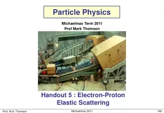
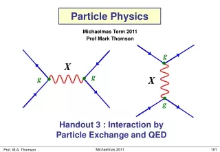
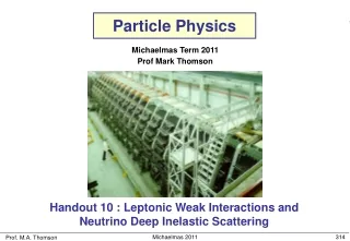
Particle Physics. Michaelmas Term 2011 Prof Mark Thomson. Handout 5 : Electron-Proton Elastic Scattering. e –. e –. e –. e –. m –. m –. Electron-Proton Scattering. In this handout aiming towards a study of electron-proton scattering as a probe of the structure of the proton.

Particle Physics
E N D
Presentation Transcript
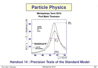
Particle Physics Michaelmas Term 2011 Prof Mark Thomson Handout 5 : Electron-Proton Elastic Scattering Michaelmas 2011
e– e– e– e– m– m– Electron-Proton Scattering • In this handout aiming towards a study of electron-proton • scattering as a probe of the structure of the proton • Two main topics: • e-p e-X deep inelastic scattering (handout 6) e-p e-pelastic scattering (this handout) • But first consider scattering from a point-like • particle e.g. e–m– e–m– i.e. the QED part of (e–q e–q) • Two ways to proceed: • perform QED calculation from scratch (Q10 on examples sheet) • take results from e+e– m+m– and use “Crossing Symmetry” to • obtain the matrix element for e–m– e–m–(Appendix I) (1) Michaelmas 2011
e– m– e– m– as the cross section tends to infinity. (2) • Work in the C.o.M: giving • The denominator arises from the propagator here Michaelmas 2011
e– e– e– e– MRR MLL MRL MLR e– e– e– e– m– m– m– m– m– m– m– m– cosq cosq cosq cosq -1 -1 -1 -1 +1 +1 +1 +1 • What about the angular dependence of • the numerator ? • The factor reflects helicity (really chiral) structure of QED • Of the 16 possible helicity combinations only 4 are non-zero: i.e. no preferred polar angle spin 1 rotation again Michaelmas 2011
e– e– p p • The cross section calculated above is appropriate for the scattering of two • spin half Dirac (i.e. point-like) particles in the ultra-relativistic limit • (where both electron and muon masses can be neglected). In this case • We will use this again in the discussion of “Deep Inelastic Scattering” of • electrons from the quarks within a proton (handout 6). • Before doing so we will consider the scattering of electrons from the composite • proton - i.e. how do we know the proton isn’t fundamental “point-like” particle ? • In this discussion we will not be able to use the • relativistic limit and require the general expression • for the matrix element (derived in the optional part of • Q10 in the examples sheet): (3) Michaelmas 2011
Probing the Structure of the Proton • In e-p e-p scattering the nature of the interaction of the virtual photon with the proton depends strongly on wavelength e– • At very low electron energies : the scattering is equivalent to that from a “point-like”spin-less object e– • At low electron energies : the scattering is equivalent to that from a extended charged object e– • At high electron energies : the wavelength is sufficiently short to resolve sub-structure. Scattering from constituent quarks e– • At very high electron energies : the proton appears to be a sea of quarks and gluons. Michaelmas 2011
e– e– (neglect proton recoil) Rutherford Scattering Revisited • Rutherford scattering is the low energy limit where the recoil of the proton can be neglected and the electron is non-relativistic • Start from RH and LH Helicity particle spinors • Now write in terms of: Non-relativistic limit: Ultra-relativistic limit: and the possible initial and final state electron spinors are: Michaelmas 2011
e– e– e– e– e– e– • In the relativistic limit ( ), i.e. e– e– • Consider all four possible electron currents, i.e. Helicities RR, LL, LR, RL (4) (5) (6) (7) (6) and (7) are identically zero; only RR and LL combinations non-zero we have • In the non-relativistic limit, All four electron helicity combinations have non-zero Matrix Element i.e. Helicity eigenstates Chirality eigenstates Michaelmas 2011
where • The initial and final state proton spinors (assuming no recoil) are: Solutions of Dirac equation for a particle at rest giving the proton currents: • The spin-averaged ME summing over the 8 allowed helicity states Note: in this limit all angular dependence is in the propagator • The formula for the differential cross-section in the lab. frame was • derived in handout 1: (8) Michaelmas 2011
This is the normal expression for the Rutherford cross section. It could have been derived by considering the scattering of a non-relativistic particle in the static Coulomb potential of the proton , without any consideration of the interaction due to the intrinsic magnetic moments of the electron or proton. From this we can conclude, that in this non-relativistic limit only the interaction between the electric charges of the particles matters. and we can neglect • Here the electron is non-relativistic so in the denominator of equation (8) • Writing and the kinetic energy of the electron as (9) Michaelmas 2011
For Rutherford scattering we are in the limit where the target recoil is • neglected and the scattered particle is non-relativistic • In this limit the electron currents, equations (4) and (6), become: Relativistic Electron “helicity conserved” Overlap between initial/final state electron wave-functions. Just QM of spin ½ Rutherford formula with The Mott Scattering Cross Section • The limit where the target recoil is neglected and the scattered particle is • relativistic (i.e. just neglect the electron mass) is called Mott Scattering • It is then straightforward to obtain the result: (10) • NOTE: we could have derived this expression from scattering of electrons in a static potential from a fixed point in space . The interaction is ELECTRIC rather than magnetic (spin-spin) in nature. • Still haven’t taken into account the charge distribution of the proton….. Michaelmas 2011
Form Factors • Consider the scattering of an electron in the static potential • due to an extended charge distribution. • The potential at from the centre is given by: with • In first order perturbation theory the matrix element is given by: • Fix and integrate over with substitution • The resulting matrix element is equivalent to the matrix element for scattering from a point source multiplied by the form factor Michaelmas 2011
There is nothing mysterious about form factors – similar to diffraction of plane • waves in optics. • The finite size of the scattering centre • introduces a phase difference between • plane waves “scattered from different points • in space”. If wavelength is long compared • to size all waves in phase and For example: Fermi function exponential Gaussian Uniform sphere point-like unity “dipole” Gaussian sinc-like Dirac Particle Proton 6Li 40Ca • NOTE that for a point charge the form factor is unity. Michaelmas 2011
Experimentally observe scattered electron so eliminate Point-like Electron-Proton Elastic Scattering • So far have only considered the case we the proton does not recoil... • For the general case is e– e– p p • From Eqn. (2) with the matrix element for this process is: (11) • The scalar products not involving are: • From momentum conservation can eliminate : i.e. neglect Michaelmas 2011
Substituting these scalar products in Eqn. (11) gives (12) • Now obtain expressions for and (13) (14) Space-like NOTE: • For start from and use Michaelmas 2011
Hence the energy transferred to the proton: (15) Because is always negative and the scattered electron is always lower in energy than the incoming electron • Combining equations (11), (13) and (14): • For we have (see handout 1) (16) Michaelmas 2011
Interpretation So far have derived the differential cross-section for e-p e-pelastic scattering assuming point-like Dirac spin ½ particles. How should we interpret the equation? • Compare with the important thing to note about the Mott cross-section is that it is equivalent to scattering of spin ½ electrons in a fixed electro-static potential. Here the term is due to the proton recoil. Magnetic interaction : due to the spin-spin interaction • the new term: Michaelmas 2011
e.g.e-p e-pat Ebeam= 529.5 MeV, look at scattered electrons at q = 75o • The above differential cross-section depends on a single parameter. For an electron • scattering angle , both and the energy, , are fixed by kinematics • Equating (13) and (15) • Substituting back into (13): For elastic scattering expect: E.B.Hughes et al., Phys. Rev. 139 (1965) B458 The energy identifies the scatter as elastic. Also know squared four-momentum transfer Michaelmas 2011
we have and So for Elastic Scattering from a Finite Size Proton • In general the finite size of the proton can be accounted for by introducing two structure functions. One related to the charge distribution in the proton, and the other related to the distribution of the magnetic moment of the proton, • It can be shown that equation (16) generalizes to the ROSENBLUTH FORMULA. with the Lorentz Invariant quantity: • Unlike our previous discussion of form factors, here the form factors are a • function of rather than and cannot simply be considered in terms of the • FT of the charge and magnetic moment distributions. But and from eq (15) obtain Michaelmas 2011
Hence in the limit we can interpret the structure functions in • terms of the Fourier transforms of the charge and magnetic moment distributions • Note in deriving the Rosenbluth formula we assumed that the proton was • a spin-half Dirac particle, i.e. • However, the experimentally measured value of the proton magnetic moment • is larger than expected for a point-like Dirac particle: So for the proton expect • Of course the anomalous magnetic moment of the proton is already evidence • that it is not point-like ! Michaelmas 2011
Measuring GE(q2) and GM(q2) • Express the Rosenbluth formula as: i.e. the Mott cross-section including the proton recoil. It corresponds to scattering from a spin-0 proton. where • At very low q2: • At high q2: • In general we are sensitive to both structure • functions! These can be resolved from • the angular dependence of the cross • section at FIXED Michaelmas 2011
q2 = 293 MeV2 E.B.Hughes et al., Phys. Rev. 139 (1965) B458 • EXAMPLE:e-p e-pat Ebeam= 529.5 MeV • Electron beam energies chosen to give certain values of • Cross sections measured to 2-3 % NOTE Experimentally find GM(q2) = 2.79GE(q2), i.e. the electric and and magnetic form factors have same distribution Michaelmas 2011
High q2 Measure Higher Energy Electron-Proton Scattering • Use electron beam from SLAC LINAC: 5 < Ebeam < 20 GeV • Detect scattered electrons using the • “8 GeV Spectrometer” bending magnets 12m e- q P.N.Kirk et al., Phys Rev D8 (1973) 63 Michaelmas 2011
Point-like proton R.C.Walker et al., Phys. Rev. D49 (1994) 5671 A.F.Sill et al., Phys. Rev. D48 (1993) 29 High q2 Results • Form factor falls rapidly with • Proton is not point-like • Good fit to the data with “dipole form”: • Taking FT find spatial charge and magnetic moment distribution with • Corresponds to a rms charge radius • Although suggestive, does not imply proton is composite ! • Note: so far have only considered ELASTIC scattering; Inelastic scattering is the subject of next handout ( Try Question 11) Michaelmas 2011
Summary: Elastic Scattering • For elastic scattering of relativistic electrons from a point-like Dirac proton: Rutherford Proton recoil Electric/ Magnetic scattering Magnetic term due to spin • For elastic scattering of relativistic electrons from an extended proton: Rosenbluth Formula • Electron elastic scattering from protons demonstrates that the proton is an extended object with rms charge radius of ~0.8 fm Michaelmas 2011
e–m–e–m– e+e– m+m– e– e– e+ m– e+e– m+m– m+ e– m– m– Appendix I : Crossing Symmetry • Having derived the Lorentz invariant matrix element for e+e– m+m– “rotate” the diagram to correspond to e–m– e–m–and apply the principle of crossing symmetry to write down the matrix element ! • The transformation: Changes the spin averaged matrix element for e–e+ m–m+ e– m–e– m– Michaelmas 2011
Take ME for e+e– m+m– (page 143) and apply crossing symmetry: (1) Michaelmas 2011