Download
1 / 54
560 likes | 789 Views
3. Climate Sensitivity and Observed Negative Feedbacks. pdf file of slides available upon request from rlindzen@mit.edu. Richard Lindzen and Roberto Rondanelli Program in Atmospheres, Oceans, and Climate, MIT.

E N D
3. Climate Sensitivity and Observed Negative Feedbacks pdf file of slides available upon request from rlindzen@mit.edu Richard Lindzen and Roberto Rondanelli Program in Atmospheres, Oceans, and Climate, MIT
Cloud and water vapor feedbacks are crucial to climate sensitivity. This talk will focus on the relevant physical processes associated with both cloud cover and water vapor, primarily as pertain to the tropics.
Preliminaries Concerning the Concepts of Climate Sensitivity and Climate Feedbacks.
It should be said at the outset, that the concept of climate sensitivity is, indeed, simplistic, and has lead to a very naïve picture of climate wherein: 1) Climate can be summarized in a single index: global mean temperature; 2) Climate is forced by net radiative change associated with changes in greenhouse gases, solar ‘constant,’ etc.; and 3) Spatial structure of climate change follows from global mean temperature. At best, such a picture might be applied to global forcing by changes in well mixed greenhouse gases, solar output, etc. It is almost certainly inappropriate to inhomogeneous forcing which acts to alter horizontal heat fluxes (Milankovitch forcing for example).
Climate sensitivity is generally defined as follows: For a doubling of CO2, DF is about 3.5 watts/m2, and if all other factors (humidity, clouds, ice and snow cover) can be held constant, the response is generally reckoned to be about 1oC; ie, Sensitivity=0.25 oC/watt/m2. The higher sensitivities, characteristic of most climate models, arise from feedbacks. Unfortunately, the above formulation of sensitivity does not allow for the convenient isolation of the role of feedbacks. Electrical engineers have developed a more appropriate formulation.
As we have just noted, G0 is generally reckoned to be about 1C for a doubling of CO2.
If, however, changes in global mean temperature elicit changes in other factors influencing the global mean temperature, we have what are called climate feedbacks. or more generally,
Clearly, our long persisting ‘official estimates’ of climate sensitivity demand positive feedbacks. These arise, in models, primarily from water vapor, clouds, and snow/ice albedo. A water vapor feedback factor of about 0.5 is common to most models, and is the largest of the three feedbacks. (Recall that water vapor and clouds are, by far, the most important greenhouse substances in the atmosphere.) The water vapor feedback was first proposed by Manabe and Wetherald (1971). They noted, using a one-dimensional model, that keeping relative humidity fixed led to a doubling of the response to increasing CO2. The point was that the same relative humidity at a higher temperature meant more water vapor, given the Clausius-Clapeyron Relation. However, the Clausius-Clapeyron Relation refers to the saturation vapor pressure, and the atmosphere is not saturated. Nevertheless, existing models behave as though relative humidity were, indeed, fixed.
Several things are worth noting about the water vapor feedback: 1. Once it is present, relatively small contributions to the feedback factor from other processes can lead to large changes in climate sensitivity. A feedback factor of 0.5 leads to a sensitivity of 2C. Adding another feedback factor of 0.5 leads to an infinite sensitivity! Thus, our uncertainty over the behavior of clouds is largely responsible for the wide range of sensitivities displayed by models -- despite the fact that their contribution (in the models) to the feedback factor is smaller than that of water vapor.
2. While one may speak of an average water vapor feedback, the nature of the water vapor budget is radically different in the tropics and in the extratropics, as is the intimate relation between clouds and relative humidity.
In the extratropics, transport is mostly by wave motions on isentropic surfaces. Rising air cools and relative humidity increases leading to saturation, condensation, and the formation of stratiform clouds. Precipitation leads to a loss of water substance. Descending air is associated with decreasing relative humidity and dryness. Nothing in this process suggests any obvious feedback (Yang and Pierrehumbert, 1994). Note that in the extratropics, high relative humidity leads to the formation of stratiform clouds (which are of primary importance to the radiative budget). In the tropics, transport is mainly due to cumulus towers, and large scale quasi-steady circulations (nominally the Hadley and Walker circulations). Regions of large scale descent are dry, and regions of large scale ascent are moist. However, ….
Within the ascending regions, the actual ascent is concentrated in the cumulonimbus towers. Air, outside these towers, is mostly descending. The air outside the towers is moistened by the evaporation of precipitation from stratiform clouds formed from the detrainment of ice from the cumulonimbus towers. Note that in the tropics, stratiform clouds lead to high humidity. Given the acknowledged poor performance of models with respect to clouds, it is surprising that it is often claimed that water vapor is well represented.
3. Water vapor is bounded by the Clausius-Clapeyron Relation, and specific humidity does decrease sharply with latitude and altitude. The fact that changes in circulation can lead to the deposition of heat at different latitudes is probably a major reason why changes in dynamics can lead to changes in global mean temperature (even without external forcing) as heat is deposited in regions with different infrared opacity. Another, of course, is the fact that the ocean is never in equilibrium with the atmosphere.
Are there any reasons to suppose that model feedbacks are wrong? There are actually quite a few, some of which we will refer to later in this talk. However, the most obvious reason to, at least, consider the possibility of negative feedbacks actually arises from the most common defense of models: namely that they replicate the record of global mean temperature.
Level of scientific understanding of factors influencing climate change Remember: Doubling CO2 give you about 3.5 Wm-2 Summary of the relative impact of different man-made and natural influences on theenvironment and their current “level of scientific understanding” (LOSU) of each Global-average radiative forcing components in 2005 • Chart taken from the IPCC’s • “Climate Change 2007: The • Physical Science Basis – • Summary for Policymakers”, • released February 2, 2007. • Quotes: • “Additional forcing factors not included here are considered to have a very low LOSU” • “Volcanic aerosols contribute an additional natural forcing but are not included in this figure due to their episodic nature” • “Range for linear contrails does not include other possible effects of aviation on cloudiness” 1 N.B. Averaging does not reflect what actual models did. 1 Not equal to simple addition of components, as uncertainty estimates are asymmetric Source: IPCC, “Climate Change 2007: The Physical Science Basis – Summary for Policymakers”
The point is simply that anthropogenic greenhouse forcing is already about 86% of that expected from a doubling of CO2, and the small warming observed is only consistent with this forcing if much of it is cancelled by uncertain aerosol forcing and ocean delay. The alternative, which is at least equally plausible is that model sensitivity is excessive. The common defense of current models is that they cannot account for recent warming at all unless there is anthropogenic forcing.
However, in what sense does the fact that a model cannot duplicate a warming of a few tenths of a degree constitute evidence that anthropogenic forcing is necessary? The alternative hypothesis is that the warming is simply natural unforced internal climate variability. It is well known that the climate does indeed fluctuate without any external forcing. There are several reasons for this. At the most fundamental level, the atmosphere and oceans are turbulent fluids, and it is a general property of such fluids that they can fluctuate widely without external forcing. There are moreover specific features of the oceans and atmosphere that lend themselves to such changes. The most obvious is that the oceans are never in equilibrium with the surface. There are exchanges of heat on all time scales between the abyssal oceans and the near surface thermocline region. Such exchanges are involved in phenomena like El Nino and the Pacific Decadal Oscillations, and produce large variable forcing for the atmosphere. In addition, the turbulent motions of the atmosphere randomly deposit heat in locations having varying water vapor and cloudiness (the two main greenhouse substances in the atmosphere) thus potentially leading to fluctuations in global mean temperature. In general, models simulate such phenomena rather poorly. Thus, it should be no surprise that they might fail to replicate a natural cause for recent warming, and this constitutes no meaningful demand for anthropogenic forcing.
Let us consider the logical alternative to the exaggerated response to greenhouse forcing: namely, that the climate models are excessively sensitive; ie, that there is an important negative feedback absent from the models. In the remainder of this talk, where I will focus on the tropics, it is necessary to keep several things in mind when observing behavior relevant to climate feedback.
1. Water vapor in the tropics is extremely spatially heterogeneous, and one dimensional treatments using spatially averaged values will almost always be misleading. So too, are results based on clear sky and cloud clearing algorithms. Instead, we suggest, feedbacks will, most likely, involve changes in the relative areas of moist/cloudy and dry/clear regions.
Both microwave and ir soundings showed that humidity varied sharply with well delineated dry and moist regions.
Studies have also shown a close coincidence of high UTH and cloud cover. This is plausible, given the origin of much tropical humidity in the evaporation of precipitation. This also suggests that stratiform clouds may serve as a surrogate for high humidity
2. Precipitation from cirrus detrained from cumulus towers is a major source of tropospheric humidity. However, the evolution of cirrus detrainment is a process which takes on the order of 6-12 hours. Given the nature of satellite orbits, this leads to statistical issues that must be handled with care.
The evaporation of the precipitation not reaching the ground is a primary source for atmospheric water vapor.
Ideally one will sample rainfall and cloud properties over a large number of systems and over complete life cycles, however this is not always possible with current observational platforms. • Stratiform and convective rainfall are not independent physical processes, if all water were rained out of the clouds in the convective towers no stratiform precipitation would be observed.
3. For climate purposes, there is a major difference between changes in cirrus associated with the concentration of convection, and changes normalized by the amount of convection. It is the latter that is relevant to climate sensitivity.
Normalization is critical to assess a global change In the context of the Bony et al (2004) methodology, a cloud property c that is “extensive” on the amount of convection (mass convective flux or precipitation) has no net “dynamical effect” if the variable that measures the amount of convection is invariant with warming (for instance P in Held and Soden (2006) is almost invariant and Mcis invariantunder a strict assumption of constant relative humidity) In order to eliminate the role of convergence in the case of local temperature, one must normalize by Mc or P.
All these issues (and more) are essential to the observational assessment of the Iris Hypothesis.
Iris Hypothesis (Lindzen et al, 2001) 3 4 2 1 1. Changes in the specific humidity of the boundary layer are mainly controlled by changes in SST. q increases at about 6-7 %/K. 2. The mean increase in q increases the liquid water content in clouds and rain processes become more efficient in the updraft regions of convective systems. 3. More efficient convective precipitation leaves less condensate (and water vapor) available for detrainment. 4. Less detrainment in turn produces a shrinkage in the cirrus coverage, in particular relatively thin cirrus that can have a net warming effect.
The original paper used geostationary infrared observations which provided continuous time coverage over a large fixed area. However, this data, like all data, had limitations. In particular, it provided only a crude measure of cumulus activity based on the area of very low infrared brightness. A better measure would be total precipitation (precipitation from both cumulus towers and from cirrus detrained from these towers). Nevertheless, the original paper suggested a strong negative feedback associated with the observation that cirrus area per unit cumulus activity decreased on the order of 10-20% per degree C. This acted to oppose warming due to the strong infrared properties of the cirrus. The negative feedback factor for the earth as a whole was on the order of -0.7 - -1.1. In this talk, I would like to concentrate on our more recent efforts.
Our work over the past year has focussed on the issue of whether we can use observations of precipitation to test for a possible increase in the efficiency of precipitation with SST. • The fraction of the convective precipitation over the life cycle of the mesoscale system can be used as a measure of the efficiency of the precipitation processes inside the convective region relative to the precipitation processes in the stratiform region. • The stratiform area normalized by the total precipitation of the system can be thought as a proxy for the total amount of detrainment
Kwajalein Radar Kwajalein is mostly an oceanic tropical site. The ground based radar provides stratiform and convective separation at 2 km pixels, based on the horizontal homogeneity of the reflectivity field. The sampling is, for practical purposes, continuous in time, with a coverage of about 150 km of radius. +
When we use the specific humidity at the surface (from soundings at Kwajalein) instead of the SST over the whole Kwajalein radar area, correlations improve (r goes from 0.39 to 0.46) . • Of course, we do expect scattering since the specific humidity in the boundary layer can hardly be the only variable controlling ε. We see that even for a well established physical relation between SST and specific humidity, there is significant scatter in this time scale, and for this particular observational setting.
Correlations are maximized in the boundary layer (ec vs. q(p))
Note that given the time dependence of the evolution of the cirrus outflow, the use of snapshots from TRMM leads to essentially random results. This is what occurred in Rapp, Kummerow et al (2005) J. Clim.
The evaporation of the precipitation not reaching the ground is a primary source for atmospheric water vapor.
Can we extend this analysis to the rest of the tropics? • Tropical Rainfall Measuring Mission (TRMM) precipitation radar (PR) measures reflectivity with high vertical resolution (~250 m). However a region equivalent to the Kwajalein radar area is visited by the satellite only once every ~ 3 days. • Sampling errors for the quantities e and A_s can be calculated by resampling the Kwajalein radar dataset at the satellite visit frequency. Sampling errors turn out to be smaller than the sampling errors for the monthly mean rainfall. • Other difficulties using TRMM data include attenuation at large rainfall rates and a marginal horizontal resolution for observing individual cumulus towers. This might introduce a bias in the classification of convective and stratiform pixels from the PR. (This effect is exacerbated in the passive microwave imager)
6 months in 2001 TRMM PR 5° x 5 Western Pacific 140 E – 150 W Eastern Pacific 150W – 80 W
The relatively small dependence of A_s at large SSTs does not seem consistent with the Kwajalein radar. We have approached this by studying TRMM PR data that overlaps Kwajalein radar data. The relations are robust to reasonable changes in the Z-R relations used to calculate precipitation and also to changes in the parameters of the classification algorithms.
One of the most noticeable di®erences is the higher sensitivity of the KR which appears in the histogram as a KR stratiform distribution extending towards values smaller than 0.1 mmh¡1 whereas the PR stratiform distribution begins abruptly at about 0.2 mmh¡1 coincident with the lower threshold in re°ectivity of the TRMM-PR instrument of about 17dBZ. Also, the mode of the convective precipitation distribution is located at a lower rainfall rate for TRMM probably a consequence of the larger pixel size in the PR (4.3 km compared to 2 km for KR). For the same reason the KR has a higher frequency of high rainfall rates than TRMM.
The convective stratiform algorithm is applied to the reflectivity data before it has been corrected for attenuation, and therefore this might result in a misclassifcation of some convective echoes into stratiform. This can be exacerbated by the instrument resolution of 4 km which is only partially adequate to distinguish single convective cells (Houze (1993) indicates that most of the single updrafts have diameters from 1 to 5 km) compared to the 2 km resolution of the Kwajalein radar. The misclassification of convective pixels into stratiform due to attenuation, pixel resolution and sensitivity all point in the same direction. Convective rainfall rates are smaller in PR than KR and for high rainfall rates in the warmer end of the correlations this results in a major over estimation of As for small values as shown if Fig. 5.
Summary of Preceding Results • The amount of convective precipitation increases faster with SST than the amount of stratiform precipitation. • The area of stratiform rainfall per unit of total precipitation decreases by about 10%/K to 25 %/K . • Results are quantitatively similar for these two independent datasets (Kwajalein Radar, TRMM-PR) when Z-R relations, classification algorithms, and differences in the measurements are accounted for. • Our metrics do not answer the question of whether the Iris effect is the explanation behind the long term trends in OLR and SW observed in the tropics, rather they show that observations are consistent with an increase in the precipitation efficiency in convective regions of the mesoscale convective systems.
There are, nonetheless, reasons to suppose that the area of stratiform rain is indicative of the total stratiform area, and that the observed decadal changes in OLR do represent negative feedbacks of the same magnitude predicted by the Iris Effect.
The studies we have shown have looked at the area of stratiform rainfall. The original study (Lindzen, Chou and Hou, 2000) looked at the area within specific ir brightness contours. In both cases, it was unclear as to whether these measures were appropriate to the total cirrus outflow. However, the recent work of Choi and Ho (2006, Radiative effect of cirrus with different optical properties over the tropics in MODIS and CERES observations, GRL, 33, L21811) shows that cirrus distributions are fairly universal, with a dominance of ir radiative impact.
In addition, numerous studies have identified ‘anomalous’ OLR in the 90’s as opposed to the 80’s:
Chen, J., B.E. Carlson, and A.D. Del Genio, 2002: Evidence for strengthening of the tropical general circulation in the 1990s. Science, 295, 838-841. Del Genio, A. D., and W. Kovari, 2002: Climatic properties of tropical precipitating convection under varying environmental conditions. J. Climate, 15, 2597–2615. Wielicki, B.A., T. Wong, et al, 2002: Evidence for large decadal variability in the tropical mean radiative energy budget. Science, 295, 841-844. Lin, B., T. Wong, B. Wielicki, and Y. Hu, 2004: Examination of the decadal tropical mean ERBS nonscanner radiation data for the iris hypothesis. J. Climate, 17, 1239-1246. Cess, R.D. and P.M. Udelhofen, 2003: Climate change during 1985–1999: Cloud interactions determined from satellite measurements. Geophys. Res. Ltrs., 30, No. 1, 1019, doi:10.1029/2002GL016128. Hatzidimitriou, D., I. Vardavas, K. G. Pavlakis, N. Hatzianastassiou, C. Matsoukas, and E. Drakakis (2004) On the decadal increase in the tropical mean outgoing longwave radiation for the period 1984–2000. Atmos. Chem. Phys., 4, 1419–1425. Clement, A.C. and B. Soden (2005) The sensitivity of the tropical-mean radiation budget. J. Clim., 18, 3189-3203.
This ‘anomaly’ is quantitatively greater than what one would expect from the iris effect (that is to say, represents a larger negative feedback)(Chou and Lindzen (2002) Comments on “Tropical convection and the energy balance of the top of the atmosphere.” J. Climate, 15, 2566-2570.), but, except for the last paper, all attempted to argue a different origin for the observation. The last showed that the alternative explanations were inconsistent with existing models. Recently, Wong et al (Wong, Wielicki et al, 2006, Reexamination of the Observed Decadal Variability of the Earth Radiation Budget Using Altitude-Corrected ERBE/ERBS Nonscanner WFOV Data, J. Clim., 19, 4028-4040) have reassessed their data to reduce the magnitude of the anomaly, but the remaining anomaly still represents a substantial negative feedback, and there is reason to question the new adjustments. For example, a more recent examination of the same datasets explicitly confirms the iris relations at least for intraseasonal time scales (Spencer, R.W., W.D. Braswell, J.R. Christy and J. Hnilo, 2007, Cloud and radiation budget changes associated with the tropical intraseasonal oscillations, Geophys. Res. Ltrs, in press.