HEAT PROCESSES
HEAT PROCESSES. HP4. Heat transfer.


HEAT PROCESSES
E N D
Presentation Transcript
HEAT PROCESSES HP4 Heat transfer Mechanisms of heat transfer. Conduction, convection (heat transfer coefficients), radiation (example: cooling cabinet). Fourier’s law of conduction, thermal resistance (composed wall, cylinder). Unsteady heat transfer, penetration depth (derivation, small experiment with gas lighter and copper wire). Biot number (example: boiling potatoes). Convective heat transfer, heat transfer coefficient and thickness of thermal boundary layer. Heat transfer in a circular pipe at laminar flow (derivation Leveque). Criteria: Nu, Re, Pr, Pe, Gz. Heat transfer in turbulent flow, Moody’s diagram. Effects of variable properties (Sieder Tate correction for temperature dependent viscosity, mixed and natural convection). Rudolf Žitný, Ústav procesní a zpracovatelské techniky ČVUT FS 2010
Mechanisms of heat transfer HP4 • There exist 3 basic mechanisms of heat transfer between different bodies (or inside a continuous body) • Conduction in solids or stagnant fluids • Convection inside moving fluids, but first of all we shall discuss heat transfer from flowing fluid to a solid wall • Radiation (electromagnetric waves) the only mechanism of energy transfer in an empty space Aim of analysis is to find out relationships between heat flows (heat fluxes) and driving forces (temperature differences)
Heat flux and conduction HP4 General form of transport Fourier equation for temperature field T(t,x,y,z) in a solid or in a stagnant fluid taking into account internal heat sources and an adiabatic temperature increase during compression of gas. Benton
Heat flux and conduction dA HP4 Energy balance of a closed system dq = du + dw (heat delivered to system equals internal energy increase plus mechanical work done by system) tells nothing about intensity of heat transfer at the surface of system, neither about relationshipsbetween heat fluxes and driving forces (temperature gradients). This problem is a subject of irreversible thermodynamics. Intenzity of heat transfer through element dA of boundary is characterized by vector of heat flux [W/m2] Direction and magnitude of heat flux is determined by gradient of temperature and thermal conductivity of media Fourier’s law of heat conduction Heat flow through boundary is projection of heat flux to the outer normal
Thermal conductivity HP4 Thermal and electrical conductivities are similar: they are large for metals (electron conductivity) and small for organic materials. Temperature diffusivity a is closely related with the thermal conductivity Memorize some typical values: Thermal conductivity of nonmetals and gases increases with temperature (by about 10% at heating by 100K), at liquids and metals usually decreases.
Conduction – Fourier equation dA HP4 Distribution of temperatures and heat fluxes in a solid can be expressed in differential form, based upon enthalpy balancing of infinitesimal volume dv Integrating this differential equation in a finite volume V the integral enthalpy balance can be expressed in the following form using Gauss theorem Accumulation of enthalpy in unit control volume Divergence of heat fluxes (positive if heat flows out from the control volume at the point x,y,z) Heat transferred through the whole surface S Accumulation of enthalpy in volume V
Conduction – Fourier equation important! HP4 Heat flux q as well as the enthalpy h can be expressed in terms of temperatures, giving partial differential equation – Fourier equation Internal heat source (e.g. enthalpy change of a chemical reaction or a volumetric heat produced by passing electric current or absorbed microwaves) Thermal conductivity need not be a constant. It usually depends on temperature, and for anisotropic materials (e.g. wood) it depends also on directions x,y,z – in this case ij should be considered as the second order tensor.
Conduction - stationary HP4 Let us consider special case: Solid homogeneous body (constant thermal conductivity and without internal heat sources). Fourier equation for steady state reduces to the Laplace equation for T(x,y,z) Boundary conditions: at each point of surface must be prescribed either temperature T or the heat flux (for example q=0 at an insulated surface). Solution ofT(x,y,z) can be found for simple geometries in an analytical form (see next slide) or numerically (using finite difference method, finite element,…) for more complicated geometry. The same equation written in cylindrical and spherical coordinate system (assuming axial symmetry)
Example temperature profile in a cylinder HP4 Calculate radial temperature profile in a cylinder and sphere (fixed temperatures T1 T2 at inner and outer surface) R1 R2 cylinder Sphere (bubble)
Conduction – thermal resistance Q T2 T1 T1 T2 T2 S2 R2 S h R1 T1 T2 S1 R1 T1 L L h h1 h2 HP4 Knowing temperature field and thermal conductivity it is possible to calculate heat fluxes and total thermal power Qtransferred between two surfaces with different (but constant) temperatures T1 a T2 RT[K/W] thermalresistance In this way it is possible to express thermal resistance of windows, walls, heat transfer surfaces … SerialParallel Tube wall Pipe burried under surface
Conduction - nonstacionary HP4 Time development of temperature field T(t,x,y,z) in a homogeneous solid body without internal heat sources is described by Fourier equation with the boundary conditions of the same kind as in the steady state case and with initial conditions (temperature distribution at time t=0). This solution T(t,x,y,z) can be expressed for simple geometries in an analytical form (heating brick, plate, cylinder, sphere) or numerically. The coefficient of temperature diffusivity a=/cpis the ratio of temperature conductivity and thermal inertia
Theory of penetration depth Tw important! t+t t x T0 δ +Δ HP4 Development of temperature profile in a half-space. Use the acceptable approximation by linear temperature profile Integrate Fourier equations (up to this step it is accurate) Approximate temperature profile by line Result is ODE for thickness as a function of time Using the exact temperature profile predicted by erf-function, the penetration depth slightly differs =(at)
Theory of penetration depth HP4 =at penetration depth. Extremely simple and important result, it gives us prediction how far the temperature change penetrates at the time t. This estimate enables prediction of thermal and momentum boundary layers thickness etc. The same formula can be used for calculation of penetration depth in diffusion, replacing temperature diffusivity a by diffusion coefficient DA . Wire Cu =0.11 m =398 W/m/K =8930 kg/m3 Cp=386 J/kg/K
Convection HP4 General form of transport Fourier Kirchhoff equation Benton
Convection Boiling (bubbles) ,y dA Outer flow-thermal boundary layer HP4 Calculation of heat flux q from flowing fluid to a solid surface requires calculation of temperature profile in the vicinity of surface (for example temperature gradients in attached bubbles during boiling, all details of thermal boundary layer,…). Engineering approach simplifies the problem by introducing the idea of stagnant homogeneous layer of fluid, having an equivalent thermal resistance (characterized by the heat transfer coefficient [W/(m2K)]) Tf is temperature of fluid far from surface (behind the boundary of thermal boundary layer), Twis wall temperature. Thickness of stagnant boundary layerδ, f thermal conductivity of fluid. Tf Tf
Example heating sphere HP4 It is correct only as soon as the heat flux q or the temperature is uniform on the sphere surface Temperature distribution inside a solid sphere Boundary condition (convection) Heat flux calculated from Fourier law inside the sphere equals the flux in fluid Fourier equation can be integrated at the volume of body (sphere in this case) The integrals can be evaluated by the mean value and by Gauss theorem, assuming uniform flux at the surface
Example heating sphere HP4 For the case that the temperature inside the sphere is uniform (as soon as the thermal conductivity s is very high) the mean temperature is identical with the surface temperature This exponential solution works only for small values of Biot number Thermal resistance of fluid >> thermal resistance of solid
Convection – Nu,Re,Pr important! HP4 Heat transfer coefficient depends upon the flow velocity (u), thermodynamic parameters of fluid () and geometry (for example diameter of sphere or pipe D). Value is calculated from engineering correlation using dimensionless criteria Nusselt number(dimensionless , reciprocal thickness of boundary layer) Reynolds number(dimensionless velocity, ratio of intertial and viscous forces) Prandl number(property of fluid, ratio of viscosity and temperature diffusivity) Rem: is dynamic viscosity[Pa.s], kinematic viscosity[m2/s], =/ And others Pe=Re.Pr Péclet number Gz=Pe.D/L Graetz number (D-diameter, L-length of pipe) Rayleigh De=Re√D/Dc Dean number (coiled tube, Dcdiameter of curvature)
Convection in a pipe HP4 Basic problem for heat transfer at internal flows: pipe (developed velocity profile) and a constant wall temperature Liquid flows in a pipe with the constant wall temperature Twthat is different than the inlet temperature T0. Temperature profile depends upon distance from inlet and upon radius r (only thin temperature boundary layer of fluid is heated). Heat flux varies along the pipe even if the heat transfer coefficient is constant, because driving potential – temperature difference between wall and the bulk temperature Tmdepends upon the distance x. Tmis the so called mean calorific temperature Heat flux from wall to bulk ( is related to the calorific temperature as a characteristic fluid temperature at internal flows)
Convection in a pipe Q Tw T0 Tm D x dx HP4 Axial temperature profile Tm(x) follows from the enthalpy balance of system, consisting of a short element of pipe dx : Solution Tm(x) by integration
Convection in a pipe HP4 • Previous integration is correct only if and the wall temperature are constant. • This doesn’t hold in laminar flow characterized by gradual development of thermal boundary layer (at entry this layer is thin and therefore=/ is high, decreases with increasing distance). Typical correlations for laminar flow • is almost constant at turbulent flows characterized by fast development of thermal boundary layer. Typical correlation (Dittus Boelter) • More complicated are cases with mixed convection (effect of temperature dependent density and gravity), variable viscosity and first of all influence of phase changes (boiling/condensation). Leveque Haussen general formula for variable wall temperature and variable heat transfer coefficient Q Tw T0 D Toutlet L
Convection Laminar Leveque Tw T0 y D umax x HP4 Leveque method is very important technique how to estimate thickness of thermal boundary layer and the heat transfer coefficient in many internal flows (not only in circular pipes). This theory is applicable only for “short” channels, in the region of developing temperature profile. velocity at bouindary layer time of penetration Graetz number Gz=Re.Pr.D/L
Mixed convection, Sieder Tate HP4 • Temperature dependendent properties of fluid are respected by correction coefficients applied to a basic formula (Leveque, Hausen, …similar corrections are applied in correlations for turbulent regime) • Temperature dependent viscosity results in changes of velocity profiles. In case of heating the wall temperature is greater than the bulk temperature, and viscosity of liquid at wall lowers. Velocity gradient at wall increases thus increasing heat transfer (look at the derivation of Leveque formula modified for nonnewtonian velocity profiles). Reversaly, in case of cooling (greater viscosity at wall) heat transfer coefficient is reduced. This effect is usually modeled by Sieder Tate correction (ratio of viscosities at bulk and wall temperature). • Temperature dependent density combined with acceleration (gravity) generate buoyancy driven secondary flows. Resulting effect depends upon orientation (vertical or horizontal pipes should be distinguished). Intensity of natural convection (buoyancy) is characterized by Grashoff number Gr) Mixed convection (Grashoff) Sieder Tate correction Leveque
Convection Turbulent flow HP4 Boccioni
Convection Turbulent flow important! HP4 • Turbulent flow is characterised by the energy transport by turbulent eddies which is more intensive than the molecular transport in laminar flows. Heat transfer coefficient and the Nusselt number is greater in turbulent flows. Basic differences between laminar and turbulent flows are: • Nu is proportional to in laminar flow, and in turbulent flow. • Nu doesn’t depend upon the length of pipe in turbulent flows significantly (unlike the case of laminar flows characterized by rapid decrease of Nu with the length L) • Nu doesn’t depend upon the shape of cross section in the turbulent flow regime (it is possible to use the same correlations for eliptical, rectangular…cross sections using the concept of equivalent diameter – this cannot be done in laminar flows) The simplest correlation for hydraulically smooth pipe designed by Dittus Boelter is frequently used (and should be memorized) m=0.4 for heating m=0.3 for cooling Similar result follows from the Colburn analogy
Pressure drop, friction factor important! HP4 Pressure drop is calculated from Darcy Weissbach equation Friction factorfdependsupon Re and relativeroughness
Turbulent boundary layer Velocity profile Buffer layer Laminar sublayer e-roughness HP4 Rougness of wall has an effect upon the pressure drop and heat transfer only if the height of irregularities e (roughness) enters into the so called buffer layer of turbulent flow. Smaller roughness hidden inside the laminar (viscous) sublayer has no effect and the pipe can be considered as a perfectly smooth. y Dimensionless distance from wall Friction velocity Thickness of laminar sublayer is at value y+=5
Example smooth pipe HP4 Calculate maximum roughness at which the pipe D=0.1 m can be considered as smooth at flow velocity of water u=1 m/s. Blasius correlation for friction factor (smooth pipes) Thickness of laminar sublayer (y+=5)
EXAM HP4 Heat transfer (Fourier Kirchhoff transport equation explained in more details in the course Momentum Heat and Mass transfer)
What is important (at least for exam) HP4 Dimensionless criteria Nusselt Biot Fourier Reynolds Prandtl Peclet Graetz Rayleigh reciprocal thermal boundary layer thermal resistance in solid / thermal resistance in fluid dimensionless time related to the penetration time through distance D ratio of inertial and viscous forces ratio of momentum and temperature diffusivities
R2 T1 T2 R1 L What is important (at least for exam) HP4 Conduction - temperature field in solids Steady heat transfer Thermal resistance RT Unsteady heat transfer (wave of thermal disturbance) Penetration depth (distance travelled by temperature disturbance in time t)
What is important (at least for exam) HP4 Convection – heat transfer from fluid to solid (-heat transf.coef.) Forced heat transfer in a pipe Laminar flow (Leveque) Turbulent flow (Dittus Boelter) Pressure drop in pipes, effect of roughness and Moody diagram