Download

1 / 21
210 likes | 291 Views
Explore concepts like Equivalent Variation, Compensating Variation, & Consumer Surplus to measure utility & welfare changes in economics accurately. Learn about Marshallian vs. Hicksian Demand Curves & their implications.

E N D
Measuring Welfare Changes of Individuals • Exact Utility Indicators • Equivalent Variation (EV) • Compensating Variation (CV) • Relationship between Exact Utility Indicators and Consumer Surplus (CS) • How accurate an approximation of utility change is CS? See Zerbe and Dively, Chapter 5
Money Measure of Individual Utility • Each indifference curve of an individual consumer corresponds to a unique level of income • If prices are fixed! • The change in utility of an individual from a policy that provides a direct cash transfer, without changing any prices, can be measured by the value of the transfer
Indifference Curves X2 M2 M1 M0 U3 U2 U1 U0 X1
Equivalent Variation • Consider an action which will cause a price to change. • This price change will change the utility of the consumer
Equivalent Variation • How much money would have to be given to or taken away from the consumer to give them the equivalentutility of the proposed action. • Consumer moves to new utility level, but the action not undertaken (prices do not change)
Equivalent Variation Y EV U1 U0 P1 P0 X
Compensating Variation • After introducing a change, how much money would have to be given to or taken away from a consumer (compensation) to place them at their original level of utility • Action is undertaken but income provided to or taken away to place the consumer at the previous level of utility. (prices do change)
Compensating Variation Y CV U1 U0 P1 P0 X
Equivalence of EV and CV EV for price decrease = CV for price increase CV for price decrease = EV for price increase
EV for a Price Decrease Y EV U1 U0 P1 P0 X
CV for a Price Increase Y CV U0 U1 P0 P1 X
Marshallian vs Hicksian Demand Curves • Marshallian demand curve: • Shows quantities demanded for different price levels, holding money income constant. • Slutsky decomposition of effect of a price change: • Pure substitution effect • Income effect
Marshallian vs Hicksian Demand Curves • Hicksian, or compensated demand curve • Shows quantities demanded at different price levels, holding utility constant. • Only the pure substitution effect • Smaller response to price change (less elastic), than Marshallian demand curve - for normal goods.
Marshallian and Hicksian Demand Curves Y Price decrease U1 U0 P1 P0 X X0 X1H X1M
Marshallian and Hicksian Demand Curves Price decrease Px P0 x P1 x x DM DH X0 X1H X1M Qx
Marshallian and Hicksian Demand Curves Y Price Increase U0 U1 P0 P1 X X1M X1H X0
Marshallian and Hicksian Demand Curves Price Increase Px P1 x x P0 x DM DH X1M X1H X0 Qx
Marshallian and Hicksian Demand Curves Px P1 P0 DM DH|U(P1) DH|U(P0) Qx
CV, EV, & CS • CV and EV are measured on Hicksian (compensated) demand curves • CS is measured on Marshallian demand curve • CS is only approximation of welfare change • It is “average between CV and EV • Willig – under wide range of conditions CS is close approximation of CV, EV.
Marshallian and Hicksian Demand Curves Px P1 CV EV CS P0 DM DH|U(P1) DH|U(P0) Qx
Comparison of CS, EV CV • Empirically, we are able to estimate CS, but not EV or CV. • How close an approximation is CS to EV or CV? • Depends on magnitude of the income effect • Differences are small for small price changes • Differences are small if (Marshallian) demand curve is inelastic