
Ordinal Optimization for Simulation-Based Performance Evaluation
E N D
Presentation Transcript
Ordinal Optimization— Soft Optimization for Hard Problems — Qing-Shan Jia (贾庆山) Email: jiaqs@tsinghua.edu.cn Lecturer Center for Intelligent and Networked Systems (CFINS) Dept. of Automation, Tsinghua University, Beijing 100084, China
Acknowledgment • Joint work with • Prof. Yu-Chi Ho(何毓琦) • Prof. Qian-Chuan Zhao(赵千川) • Prof. Xiao-Hong Guan(管晓宏) • Dr. Chen Song(宋宸) • Supported by • National Science Foundation, China • New Century Excellent Talents in University, China • 973 fundamental research grants, China • Army Research Office • Air Force Office of Scientific Research
Outline • Background: simulation-based optimization • Ordinal optimization • Comparison of selection rules • Constrained ordinal optimization • Vector ordinal optimization • Application Example • Performance optimization in a remanufacturing system • Conclusion
Human-made complex systems Transportation system Manufacturing system Electric power grid Communication system Supply chain
Major difficulties • Simulation-based performance evaluation • Time-consuming simulation • Noisy observation • Discrete parameters • Large design space: curse of dimensionality • No gradient information
Ordinal Optimization (OO) • OO is an important tool to deal with simulation-based optimization. • First developed by Prof. Y.-C. Ho, R. S. Sreenivas, and P. Vakili in 1992 [Ho, Sreenivas and Vakili1992]. • In the past decade, more than 200 publications and many successful applications. • An online incomplete OO publications list is available at: http://www.cfins.au.tsinghua.edu.cn/en/resource/index.php • The first book on OO is upcoming: • Ho, Y.-C., Zhao, Q.-C., and Jia, Q.-S., Ordinal Optimization: Soft Optimization for Hard Problems, Springer, 2007, to appear.
Basic ideas (I) • Ordinal comparison v.s. • Which one is heavier? • How much heavier, say in unit of oz. or gram? • It is easier to find out which design is better than to answer how much better.
Basic ideas (II) • Goal softening v.s. • Which board is easier to hit? Why? • It is easier to find a good enough design than to find the optimal design.
Basic ideas - summary • Ordinal comparison • Compare designs using a crude model, computationally fast but rough performance estimate. • Goal softening • Finding the global optimal is practically infeasible. A more reasonable goal: find a good enough (top-n%) design. • Not only intuitively reasonable, but also can be shown in a mathematically rigorous way • Observed order converges to true order exponentially fast w.r.t. # of observations [Dai1996, Xie1997]. • The probability that some of the observed top-n% designs are truly good enough converges to 1 exponentially fast w.r.t. n [LeeLauHo1999]. • Instead of finding the best for sure, OO finds a good enough design with high probability. • What do we save in this way? And how much?
Application Procedure Q:design space G:good enough set S:selected set :true optimum :estimated optimum Pr{|GS|k} : alignment probability Q G S k
Demonstration • 200 designs • True performance J(qi)=i, i=1,2…200. • Observed performance • i.i.d. uniformly distributed noise U[0,W]. • Question: How many observed top-12 (6%) designs are truly top-12 on the average? • …demonstration…
Demonstration - summary • W=100, Pr{|GS|3}0.95. |GS|≈5 on average. • W=10000 (Blind Pick), |GS|≈1 on average. • |GS| is robust w.r.t. noise. • The crude model helps to find some good enough designs, and saves the computing budget by one order of magnitude (from 200 to 12).
Problem type • For a given g, k, noise level, and problem type, the value of s can be calculated using a table in [LauHo1997], s.t. Pr{|GS|k} 0.95.
OO Summary • Step 1: random sample N designs from Q • Step 2: user defines g and k. • Step 3: evaluate the designs using a crude model • Step 4: estimate the noise level and problem type • Step 5: calculate the value of s s.t. Pr{|GS|k} 0.95. • Step 6: select the observed top-s designs • Step 7: OO theory ensures there are at least k truly good enough designs in S with high probability. • Usually saves the computing budget by at least one order of magnitude. • Useful to fast screen out some good enough designs, and easily combined with other optimization methods.
Selection rules • Blind Pick • Horse Race • Motivated by sports games • Pair-wise elimination as in U.S. Tennis Open • Round Robin as in NBA season games Round 1: q1 vs. q2, q3 vs. q4 Round 2: q1 vs. q3, q2 vs. q4 Round 3: q1 vs. q4, q2 vs. q3
Selection rules - continued • Optimal Computing Budget Allocation (OCBA): not to waste on bad designs. distinguish the truly best from the rest designs. • Breadth vs. Depth: automatic balance between exploration and exploitation
Comparison • Question: Which selection rule needs to select the smallest S s.t. Pr{|GS|k}0.95? • Theoretical study and abundant experiments • We find easy ways to predict a good selection rule when the problem is given. • Also some properties of good selection rules. • Some quick and dirty rules: • Horse Race is in general a good selection rule.
Constrained Ordinal Optimization • Simulation-based constraints: E[Ji(q)]0 Directly apply OO Constrained OO Estimated feasible designs Q G G S S Many infeasible designs Less infeasible designs
COO - continued • Basic idea: Use a feasibility model to screen out the feasible designs first, with a small probability to make mistakes. • Then apply OO in the set of estimated feasible designs. • Requires a smaller selected set than directly applying OO without a feasibility model. • The size of the selected set also depends on the accuracy of the feasibility model. Formula were also obtained [Guan, Song, Ho, Zhao 2006].
2nd Layer 1st Layer Vector Ordinal Optimization • Multi-objective simulation-based optimization • What is the order among designs? • The concept of layers 1st Layer: Pareto Frontier Designs with in the same layer are incomparable. Designs with a smaller layer index are better. Good enough set: designs in the first n layers. Selected set: designs in the observed first n layers. 3rd Layer
Problem type Hard Neutral Easy True performance # of designs in each layer # of designs in the first x layers
VOO - continued • The relationship between g, s, k, noise level, and problem type has also been tabularized [Zhao, Ho, Jia 2005].
Aircraft Engine • Life-critical parts, expensive, failure, tear down to repair.
Remanufacturing System Parameters to optimize: Each season, # of machines in the workshop and # of parts to order in the inventory. Objective function: maintenance cost (machine cost, inventory holding cost, cost of ordering new parts) Constraint: Pr{Turn Around Time (TAT) i.e., departure time – arrival time > T0} P0
True performances Infeasible designs Feasible designs Inefficient if directly apply OO.
Application of COO • Randomly sample N=1000 designs. • Time consuming performance evaluation: 30 minutes each, 500 hours in total. • Crude model: single replication, 1.8 second each, 30 minutes in total. • A feasibility model based on rough set theory, with accuracy 98.5% [Song, Guan, Zhao, Ho 2005]. • Screen out feasible designs with small mistakes. • Then apply OO to find some feasible and truly good enough (top-5%) designs. • By reducing from N=1000 to |S|, COO saves the computing budget by at least 25 folds.
Application of VOO • Motivation: It is not clear what is the appropriate value of P0 in the constraints Pr{TAT>T0}P0. • Objective functions • J1: Pr{TAT>T0} • J2: maintenance cost • Randomly sample N=1000 designs. • G: designs in the first two layers. • S: observed top-s layers, s given by VOO theory, s.t. Pr{|GS|k}0.95.
True Performances There are 14 designs in the true first two layers.
Application of VOO - continued • For most k, VOO reduces the computing budget from N=1000 to less than 100.
Conclusion • Simulation-based optimization • Time-consuming simulation-based performance evaluation • Ordinal Optimization • Ordinal comparison • Goal softening • Use a crude model to screen out good enough designs, saves the computing budget • Horse race is in general a good selection rule. • COO: simulation-based constrains. • VOO: multi-objective simulation-based optimization.
Upcoming Book • Ho, Y.-C., Zhao, Q.-C., and Jia, Q.-S., Ordinal Optimization: Soft Optimization for Hard Problems, Springer, 2007, to appear.
Thank you! Any questions?Ask Now, or Email: jiaqs@tsinghua.edu.cn
Reference List • [Dai1996] Dai, L., “Convergence properties of ordinal comparison in the simulation of discrete event dynamic systems”, Journal of Optimization Theory and Applications, 1996, 91(2): 363-388. • [Guan, Song, Ho, Zhao 2006] Guan, X., Song, C., Ho, Y.-C., and Zhao, Q., “Constrained ordinal optimization – a feasibility model based approach”, Discrete Event Dynamic Systems: Theory and Applications, 2006, 16(2): 279-299. • [Ho, Sreenivas and Vakili1992] Ho, Y.C., Sreenivas, R. S., and Vakili, P., “Ordinal optimization of DEDS”, Discrete Event Dynamic Systems: Theory and Applications, 1992, 2(2): 61-88. • [LauHo1997] Lau, T. W. E. and Ho, Y. C., “Universal alignment probabilities and subset selection for ordinal optimization”, Journal of Optimization Theory and Applications, 1997, 93(3): 455-489. • [LeeLauHo1999] Lee, L. H., Lau, T. W. E., and Ho, Y. C., “Explanation of goal softening in ordinal optimization”, IEEE Transactions on Automatic Control, 1999, 44(1): 94-99.
Reference List contd. • [Song, Guan, Zhao, Ho 2005] Song, C., Guan, X., Zhao, Q., and Ho, Y.-C., “Machine learning approach for determining feasible plans of a remanufacturing system”, IEEE Transactions on Automation Science and Engineering, [see also IEEE Transactions on Robotics and Automation], 2005, 2(3): 262-275. • [Xie1997] Xie, X., “Dynamics and convergence rate of ordinal comparison of stochastic discrete-event systems”, IEEE Transactions on Automatic Control, 1997, 42(4): 586-590. • [Zhao, Ho, Jia 2005] Zhao, Q. C., Ho, Y. C., and Jia, Q.-S., “Vector ordinal optimization”, Journal of Optimization Theory and Applications, 2005, 125(2): 259-274.