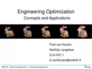
Engineering Optimization
Concepts and Applications. Engineering Optimization. Fred van Keulen Matthijs Langelaar CLA H21.1 A.vanKeulen@tudelft.nl. Summary previous lectures. Optimization problem. Responses Derivatives of responses ( design sensi- tivities ). Solving optimization problems.

Engineering Optimization
E N D
Presentation Transcript
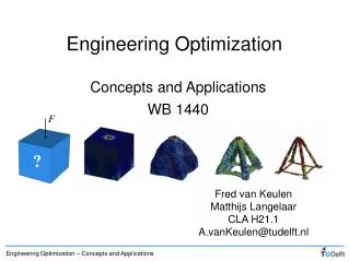
Concepts and Applications Engineering Optimization Fred van Keulen Matthijs Langelaar CLA H21.1 A.vanKeulen@tudelft.nl
Responses Derivatives ofresponses (design sensi-tivities) Solving optimization problems • Optimization problems are typically solved using an iterative algorithm: Model Constants Designvariables Optimizer
Summary Defining an optimization problem: • Choose design variables and their bounds • Formulate objective (best?) • Formulate constraints (restrictions?) • Choose suitable optimization algorithm
Positive null form: Neg. unity form: Pos. unity form: Standard forms • Several standard forms exist: Negative null form:
Multi-objective problems • Minimize c(x)s.t. g(x) 0, h(x) = 0 • Input from designer required! Popular approach: replace by weighted sum: Vector! • Optimum, clearly, depends on choice of weights • Pareto optimal point: “no other feasible point exists that has a smaller ci without having a larger cj”
Pareto set Pareto point Pareto set • Pareto point: “Cannot improve an objective without worsening another” c2 Attainable set c1
Local (rib / stiffner) level: plate thickness, fiber orientation Structural hierarchical systems • Example: wing box • Too many designvariables to treat at once • Global level: global loads, global dimensions
Optimum The design space • Design space = set of all possible designs • Example: kmax Feasible domain F k2 k2 k1 k1 kmax
Problem overconstrained: no solution exists. No feasible domain Dominated constraint (redundant) The design space (cont.)
A and B inactive A and B active B active, A inactive Objective function isolines Objective function isolines Objective function isolines Interior optimum Optimum Optimum Design space (cont.) A B
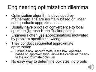
Problem characteristics • Study of objective and constraint functions: • simplify problem • discover incorrect problem formulation • choose suitable optimization algorithms • Properties: • Boundedness • Linearity • Convexity • Monotonicity
Linearity “A function f is linear if it satisfies f(x1+ x2) = f(x1)+ f(x2) andf(ax1) = af(x1) for every two points x1, x2 in the domain, and all a”
Convexity • Convex function: any line connecting any 2 points on the graph lies above it (or on it): • Linearity implies convexity (but not strict convexity)
Convexity (cont.) • Convex set [Papalambros 4.27]: “A set S is convex if for every two points x1, x2 in S, the connecting line also lies completely inside S”
Convexity (cont.) • Nonlinear constraint functions can result in nonconvex feasible domains: x2 x1 • Nonconvex feasible domains can have multiple local boundary optima, even with linear objective functions!
Feasible domain: • Convexity Optimization problem characteristics • Responses: • Boundedness • Linearity • Convexity • Monotonicity
P R t l Example: tubular column design R g3 g1 f g2 t
Optimization problem analysis • Motivation: • Simplification • Identify formulation errors early • Identify under- / overconstrained problems • Insight • Necessary conditions for existence of optimal solution • Basis: boundedness and constraint activity
f g x* x Well-bounded functions – some definitions • Lower bound: • Greatest lower bound (glb): • Minimum: • Minimizer:
Boundedness checking • Assumption: in engineering optimization problems, design variables are positive and finite • Define • Boundedness check: • Determine g+ for • Determine minimizers • Well bounded if
Examples: Bounded at zero Asymptotically bounded
l r h t Air tank design • Objective: minimize mass • Not well bounded: constraints needed
Min. head/radius ratio (ASME code): • Min. thickness/radius ratio (ASME code): • Room for nozzles:min. length • Space limitations:max. outside radius Air tank constraints • Minimum volume:
Partial minimization & bounding constraints • Partial minimization: keep all variables constant but one. Example: air tank wall thickness t: • Conclusion: • f not well bounded from below • g3 bounds t from below
A A and B active B • Activity information can simplify problem: • Active: eliminate variable • Inactive: remove constraint Constraint activity • Removing constraint = relaxing problem • Solution set of relaxed problem without gi is Xi 1. 2. 3.
f(1,x2,5) g2 g3 x2 Constraint activity checking • Example: • Conclusion: • g1 active • g2 semiactive • g3 and g4 inactive
f2 f1 x1 x2 • Similar: • Note: monotonicity convexity! • Linearity implies monotonicity Monotonicity • Papalambros p. 99: • Function f is strictly monotonically increasing if:f(x2) > f(x1) for x2 > x1 • weakly monotonically increasing if:f(x2) f(x1) for x2 > x1 • Similar for mon. decreasing
“If f(x) and gi(x) all increase or decrease (weakly) w.r.t. x, the domain is not well constrained” f(x) f g(x) x g Activity and Monotonicity Theorem • “Constraint gi is active if and only if the minimum of the relaxed problem is lower than that of the original problem” f(x) f g(x) x g2 g1
f x g First Monotonicity Principle • “In a well-constrained minimization problem every variable that increases f is bounded below by at least one non-increasing active constraint” • This principle can beused to find activeconstraints. • Exactly one boundingconstraint: critical constraint f(x) g(x)
Critical w.r.t. r Critical w.r.t. h Critical w.r.t. t Air tank design • Monotonicity analysis: What about l? Unclear.
Optimizing variables out • Critical constraints must be active:
Optimizing variables out • Critical constraints must be active:
Optimizing variables out • Critical constraints must be active:
Optimizing variables out • Critical constraints must be active:
Optimizing variables out • Critical constraints must be active:
Additional constraint from above is needed: • Maximum plate width: Problem! • Length not well bounded:
l r h t Air tank solution • Length constraint is critical: must be active! • Solution: • Result of Monotonicity Analysis: • Problem found, and fixed • Solution found without numerical optimization
Products: Products of similarly monotonic functions have: • same monotonicity if • opposite monotonicity if Recognizing monotonicity • Some useful properties: • Sums: Sums of similarly monotonic functions have the same monotonicity
Composites: Recognizing monotonicity • More properties: • Powers: Positive powers of monotonic functions have the same monotonicity, negative powers have opposite monotonicity
y • w.r.t. integrand: f1 a x b Recognizing monotonicity f1 • Integrals: • w.r.t. limits: 0 a b x
Uncritical constraint 0 Uniquely critical constraint 1 1 >1 >1 Multiple critical constraint Conditionally critical constraint Criticality Refined definitions: # of variables critically bounded by constraint i # of constraints possibly critically bounding variable j
Multiple critical constraint can obscure boundedness! Eliminate if possible Critical w.r.t. r Critical w.r.t. h Critical w.r.t. t Conditionally critical w.r.t. l Multiple critical! Air tank example
Air tank example • Starting with eliminating r:
Critical for h Critical for t Air tank example • New problem: ?
Not well bounded! Air tank example • Finally, after also eliminating h and t: • Conclusion: multiple critical constraint obscured ill-boundedness in l
Summary • Optimization problem checking: • Boundedness check of objective • Identify underconstrained problems • Monotonicity analysis • Identify not properly bounded problems • Identify critical constraints • Eliminate variables • Remove inactive constraints
x2 f 3 1 x1 Relaxed problem: But what about … • Equality constraints: • Active if all constraint variables in objective • Otherwise semi-active • Example:
More on nonobjective variables • Monotonicity Principle for nonobjective variables:“In a well-constrained minimization problem every nonobjective variable is bounded below by at least one non-increasing semiactive constraint and above by at least one non-decreasing semiactive constraint” g(x) gi gj 0 x