Download

1 / 45
450 likes | 611 Views
Inelastic cross section measurements at LHC. Rencontres du Viet Nam 14th Workshop on Elastic and Diffractive Scattering Frontiers of QCD: From Puzzles to Discoveries December 15-21, 2011 Qui Nhon, Vietnam. Marcello Bindi on behalf of ATLAS and CMS Collaborations. Outline.

E N D
Inelastic cross section measurements at LHC Rencontres du Viet Nam14th Workshop on Elastic and Diffractive Scattering Frontiers of QCD: From Puzzles to Discoveries December 15-21, 2011Qui Nhon, Vietnam Marcello Bindi on behalf of ATLAS and CMS Collaborations
Outline • Motivations • Short description of LHC and ATLAS/CMS detectors • Introduction to LHC p-p interactions • ATLAS Inelastic pp cross-section Nature Comm. 2 (2011) 463 • CMS Inelastic pp cross-section CMS-PAS-FWD-11-001 • Conclusions
Motivation for the measurement • Total proton-(anti)proton cross sections have been a fundamental quantity since the earliest days of particle physics • 20% elastic, 80% inelastic • diffractive contribution: σD /σinel ~ 0.2-0.3 • The dependence of the p-p interaction rate on the centre-of-mass collision energy √scannot yet be calculated from first principle • Common models manage to describe existing data using different methods: - Power Law (Donnachie & Landshoff) - Logarithmic (Block & Halzen) - Using aspects of QCD (Achilli et al.) • For p-p σinelat √s=7 TeV there are no good prediction due to large extrapolation uncertainties What is the contribution that LHC experiments can offer?
LHC world • The LHC is a proton-proton collider running since March 2010 at √s=7 TeV • Up to November 2011 • Peak Luminosity: • ~ 3.5·1033 cm-2s-1 • # Colliding bunches: • ~ 1300 for ATLAS/CMS • Bunch spacing: • 50 ns (75 ns during 2010) • Pile-up: • ~ 11.6 average number of • collisions/BC during 2011 • (up to 24 collisions/BC)
ATLAS: AToroidal LHC ApparatuS Three large super-conducting air-core toroidal magnets (2~6 T· m) Minimum Bias Trigger Scintillatorscover 2.09 < | η | < 3.84 Modules in front of the end-cap calorimeters (z=± 3.5m); 2 rings in η for each side, divided in 8 sectors in φ. Total weight 7000 t Overall diameter 25 m Overall length 44 m Inner Detector in 2 T axial magnetic field reconstructs charged particle “tracks” with |η| < 2.5 Electro-Magnetic (Hadronic) Calorimeters measure energy of particles with |η| < 3.2 (4.9)
CMS: Compact Muon Solenoid EM and HCAL calorimeters Total weight 12500 t Overall diameter 15 m Overall length 21.6 m Muon detectors Magnet Yoke Solenoid 3.8 T CMS η coverage: Tracker (Pixel + Strip)| η | < 2.4 Calorimeters (EM+HCAL) | η | < 3.0 HF Calorimeter 3 < | η | < 5 Muon Detectors |η| < 2.4 Inner Tracker
Dominant p-p interactions at LHC Inelastic p-p collisions are the result of a combination of non-diffractive and diffractive events: σtotal-inelastic = σND-inelastic + σSD + σDD • Non-Diffractive (ND) Single-Diffractive-Dissociation (SD) Double-Diffractive Dissociation(DD) • Pythia@7TeVσ~49 mb σ~14 mbσ~9 mb • These soft-QCD processes are needed in Monte Carlo Event Generators • To model pileup (up to ~20 extra pp interactions per bunch crossing) • To model the soft processes occurring in the same pp interaction as an “interesting” event
Measurement of the Inelastic Proton-Proton Cross-Section at √s=7 TeV with the ATLAS Detector
ATLAS Inelastic cross section: preamble on detector acceptance • Direct measurement of σinel using Minimum Bias trigger • Blind to events with all the particles at| η | > 3.84, (mostly diffractive events) • x=M2X/s , where M2X is calculated for the most spread set of hadrons • x relates to rapidity gap size inside the detector acceptance: ηMinlog (1/x) • x > 5x10⁻⁶ • (MX >15.7 GeV for √s=7 TeV)
ATLAS Inelastic cross section: definition of fiducial cross section Correction factors taken from MC, detector response tuned to Data Detectable
ATLAS Inelastic cross section: event selection and background • Trigger requirements: at least one hit in the MBTS counters very efficient w.r.t. to the offline selection: trig=99.98% • Offline selection: ≥ 2 MBTS hits, counter’s charge > 0.15 pC (noise ~ 0.02 pC) Inclusive sample - for the actual cross section measurement: • ≥2 counters above threshold in the whole detector 1.2 M events at 7 TeV in a single run (~20 µb-1) Single-sided sample - to be able to constrain the diffractive contribution: • ≥ 2 counters above threshold on one side, none on the opposing side 120 K events at 7 TeV in a single run (~20 µb-1) Background estimation coming from direct beam interactions with gas in the beam- pipe, beam-pipe itself and material upstream the detector (single proton bunch) and from “afterglow”, like slowly decaying beam remnants (timing distribution) ≤ 0.4%
ATLAS Inelastic cross section: relative diffractive contribution • Measure the ratio of the single-sided to inclusive event sample Rss • Compare with predictions (from several models) ofRss as a function of an assumed • value of fD(fractional contribution of diffractive events to the inelastic cross-section) • Default fD = 32.2% for all models but • Phojet (20.2%) • Constrain fD such that it reproduces • the measured Rss • fD = 26.9+2.5-1.0 % (fromDonanchie & Landshoff) • Systematic uncertainties: • propagated from Rss , by variating • the ratio SD/DD Rss = [10.02 ± 0.03(stat.)i+0.1−0.4(sys.)]%
ATLAS Inelastic cross section: efficiency determination • sel= fraction of event in the kinematic range (x > 5x10⁻⁶ ) that pass the selection • Single-sided sample choose as benchmark for the MC • Data best described by Donnachie & Landshoff (DL) model (ε = 0.085, α‘ = 0.25 GeV-2) ↪ Taken as the default model for the efficiency estimate • MBTS hit multiplicity distribution in the data compared with MC expectations for several MC models using the fitted fD values. sel= 98.77% • Very low migration into the fiducial region: f(ξ < 5 × 10⁻⁶) = 0.96 % • Spread among models considered: < 0.5%
ATLAS Inelastic cross section: efficiency determination • MBTS hit multiplicity distribution in the inclusive sample compared with MC expectations for several MC models using the fitted fD values : for low multiplicities, data is within the various predictions. • Systematic uncertainty due to: • Fragmentation difference • between Pythia6 and Pythia8: 0.4% • x dependence: maximum deviation of • default model DLε=0.085, α‘=0.25 GeV-2 • from the other DL models: 0.4% • MBTS detector response and the amount • of material in front of the MBTS detector • lead to systematic uncertainties on data
ATLAS Inelastic cross section:cross section and uncertainties Calculate fiducial cross-section using: sel= 98.77% trig = 99.98% fξ<5x10-6= 0.96% Lumi =20.25 μb-1 • Statistical uncertainty negligible (±0.05 mb) 0.08% • Luminosity is the dominant sys. uncertainty • Measured using dedicated Van der Meer scans • Limited by bunch current measurement • Very efficient and well understood trigger • Detector response in general well modeled (~2%), differences corrected for in the MC • Conservative estimate of beam backgrounds 0.4% correction factor (Pythia6/8)
ATLAS Inelastic cross section: • extrapolation to total inelastic • Comparison with analytic theoretical calculations or other measurements • Fraction of events in the selected fiducial region depends on the x • evolution of the cross section • Extrapolation via using DL (default) • 87.3 % of the total cross section • within the kinematic acceptance • Other models go from 79% • (Ryskin et al.) to 96% (PHOJET) • +/-10% as extrapolation uncertainty Extrapolation
ATLAS Inelastic cross section:results Extrapolated down to x=m2p/s using Pythia • Data (x > 5x10⁻⁶) significantly lower than MC predictions from both S&S and PHOJET • Uncertainty dominated by absolute luminosity calibration • Extrapolated value agrees with models (power law, logarithmic rise,..) within uncertainties dominated by uncertainty on the x-dependence of
Measurement of the inelastic pp cross section at √s = 7 TeV with the CMS detector
CMS Inelastic cross section: preamble • New method based on the assumption that the number of inelastic p-p interactions • in a given bunch crossing (# pile-up events) follows the Poisson probability • distribution: • nPileupdepends on the total σ(pp) cross sectionandon the luminosity L , • where L=Lbx(luminosity per bunch crossing), known with a precision of 4% • cross-checked using the number of triggers in each bunch (L* σ = Nevents) • • Pile up events are recorded by a high efficient and stable trigger (double ee, pT > 10 • GeV); important that trigger efficiency does not depend on nPileup • • The goal of the analysis is to count the number of primary vertexes (nPileup ) as a • function of luminosity (Lbx) to extract σ
CMS Inelastic cross section: analysis procedure 1. Acquire the bunch crossing (BC) using a primary event: the BC is recorded because of a firing trigger. Primary event used “only“ to record the BC producing an unbiased sample 2.Count the number of pile-up (PU) events: for any BC count the number of vertices in the event. 3.Correct the number of visible vertices for various effects: vertex merging, vertex splitting, real secondary vertices… 4.Fit the probability of having n = 0,….8 pile-up events as a function of luminosity: using a Poisson fit for each bin 9 values of σ(pp)n 5.Fit the 9 values together: from σ(pp)nwe obtain σ(pp)
CMS Inelastic cross section: • vertex requirement and efficiency • Track requirements : ( 2 pixel hits) && (5 strip hits) • Vertex requirements : (2 tracks) && (pT>200 MeV) && (|η|<2.4) • Vertex quality cut : NDOF>0.5 Fake vertices contamination (~ 1.5 10-3): - real secondary vtxs (long lived particles) - fake secondary vtxs (vtx alg. splitting a single vtx) • • Tracker GEANT simulation used to compute the vertex • reconstruction efficiency • • Algorithm reconstructs vertices separated by ≥ 0.06 mm. • The “blind distance” is largely independent of the • number of tracks in the vertexes • Need to correct PU distribution for the missing fraction • of events at low multiplicity and for vertex merging effect
CMS Inelastic cross section: count the number of PU events • LHC has reached a peak luminosity of • 2*1032 cm-2 s-1 for this 2010 analysis • However, the important parameter is the • luminosity per bunch crossing • an accurate measurement needs a large • luminosity interval: 0.05 0.7 ·1030cm-2s-1 Data divided into 13 luminosity bins In each luminosity bin the number of vertices is computed Analyzed events with 0-8 PU events Ratio Data/MC very flat up to 8 pile-up events nPU = # vertices-1
CMS Inelastic cross section: • corrected distributions Using the correction functions, we unfold the measured vertex distributions to obtain the correct distributions to fit with a Poisson function: Events with 1 pile-up Events with 0 pile-up Events with 3-8 pile-up Events with 2 pile-up
CMS Inelastic cross section: fitted cross sections From the fit to each distribution σ(pp)n with n=1,..9 being the number of vertices. A fit to these 9 values gives the final value: σ(pp ) = 58.7 mb (2 charged particles, pT>200 MeV, |η|< 2.4) x (x=M2X/s) interval: > 6 *10-5
CMS Inelastic cross section: main systematic checks • Variation of the luminosity values: • CMS luminosity value known with a precision of 4% σ = 2.4 mb • Modification of some analysis parameters: • Different set of primary events (single mu/double el) σ = 0.9 mb • Change the Poisson fit limit by 0.05·1030σ = 0.2 mb • Change the minimum distance between vertices • from 0.1 cm to 0.06 and 0.2 cm σ= 0.3 mb • Change the vertex quality requirement (NDOF 0.1 – 2) σ= 0.3 mb • Vertex Transverse position cut (0.05-0.08 cm) σ= 0.3 mb • Number of minimum tracks at reconstruction σ = 0.1 mb • Use the analytic method • Use the analytic method instead of a MC σ = 1.4 mb • σ(pp ) = 58.7 ± 2.0 (Syst) ± 2.4 (Lumi) mb σ = 1.4 mb
CMS Inelastic cross section: MC models and extrapolation • Comparison between the CMS results and several Monte Carlo models • CMS Systematic uncertainties (inner red error bars) and luminosity • uncertainty (outer black bars) • Monte Carlo predictions • with a common • uncertainty of ~1 mb • Except PHOJET and • SIBYLL (overestimating), • QGSJET (too high), the • other models agree (2 ) • used for extrapolation!
CMS Inelastic cross section: results inel = 68 ± 2.0 (syst.) ± 2.4(lumi) ± 4. (extr.) mb
ATLAS and CMS comparison between them CMS (x > 6x10⁻⁵ ) = 58.7 ± 2.0 (sys) ± 2.4 (lum) mb ATLAS (x > 5x10⁻⁶) = 60.3 ± 0.5 (sys.) ± 2.1 (lum) mb CMS inel = 68.0 ± 2.0 (sys.) ± 2.4(lum) ± 4. (extr.) mb ATLAS inel = 69.1 ± 2.4 (exp.) ± 6.9 (extr.) mb
Total and Inelastic p-p cross section at LHC • ATLAS and CMS central values lower than TOTEM after extrapolation • into region of very low ξ (extrapolation error is dominant)
Conclusions • ATLAS and CMS have performed precise (3.5-5%) measurements of the fiducial inelastic proton-proton cross section for LHC at √s 7 TeV • Both measurements are dominated by the absolute luminosity calibration (3.5-4%) • ATLAS results are significantly below predictions by PHOJET and Schuler & Sjöstrand(Pythia); CMS finds a similar discrepancy for PHOJET but a smaller discrepancy with Pythia respect to ATLAS • ATLAS and CMS total inelastic cross section both suffer from uncertainties on the ξ-dependence that imply a large extrapolation error. • The results are consistent with predictions from Pythia (power law dependence on √s), from Block & Halzen (logarithmic dependence) and from other theoretical calculation (Ryskin et al., Achilli et al.)
Dominant p-p interactions at LHC • The pp inelastic cross-section is much larger than that for “new” particle production only 1/109 interactions would produce a Higgs • p-p dominated by soft QCD (low-pT transfer): • Initial and final state radiations • Colour recombination • Multiple Parton Interactions (MPI) • Underlying events… • Soft QCD processes are unavoidable background for jet cross sections, missing energy, isolation… impact on resolutions for ETmiss, jet reconstruction, lepton ID,… • Soft QCD can not be predicted using p-QCD phenomenological models are needed and Monte Carlo tunes can be tested looking for agreement with data for various observables.
ATLAS Inelastic cross section: MBTS response MBTS hit multiplicities dependent on efficiencies of single scintillators and material budget Efficiencies measured data driven: • Using extrapolated tracks with pT > 200 MeV • Calorimeter signals behind the MBTS detectors • Efficiency overestimated in the MC, by ~1% Impact of material estimated using MC with different amount of dead material, in combination with data
ATLAS Inelastic cross section: background evaluation Backgrounds from direct beam interactions with: • residual gas in the beam-pipe or the beam-pipe itself • material upstream from the detector estimate by using bunch crossings with only a single proton bunch • Inclusive selection: 0.1% • Single-sided: 0.3% Additional background from ‘afterglow‘, like slowly decaying beam remnants can be estimated from timing distributions: < 0.4%
CMS Pile-up 2011 The number of reconstructed vertices after the August Technical Stop increased by factor 1.5 (β*=1.5m 1m ) Fills start with ~15 pile-up interactions.
CMS Inelastic cross section: correct the number of vertices
Vertex merging and secondary vertices Vertex merging: When two vertexes overlap they are merged into a single one. This blind distance is ~ 0.06 cm Secondary vertices: 1.Fakes from the reconstruction program 2.Real non prompt decay Both reduced by the request on the transverse position Most evident at low track multiplicity
CMS Inelastic cross section: additional measurements Using the same technique, 4 different cross sections have been measured: • 2 charged particles with pT>200 MeV in |η|< 2.4 (pp ) = 58.7 ± 2.0 (Syst) ± 2.4 (Lum) mb • 3 charged particles with pT>200 MeV in | η |< 2.4 (pp ) = 57.2 ± 2.0 (Syst) ± 2.4 (Lum) mb • 4 charged particles with pT>200 MeV in |η|< 2.4 (pp ) = 55.4 ± 2.0 (Syst) ± 2.4 (Lum) mb • 3 particles with pT>200 MeV in |η|< 2.4 (pp ) = 59.7 ± 2.0 (Syst) ± 2.4 (Lum) mb
Minimum Bias Events (from CSC book) Central charged particle density for non-single diffractive inelastic events as a function of energy. The lines show predictions from PYTHIA using the ATLAS tune and CDF tune-A, and from PHOJET. The data points are from UA5 and CDF p-(anti)p data.
Minimum Bias Events (from CSC book) Pseudorapidity (a) and transverse momentum distribution (b) of stable charged particles from simulated 14TeV pp inelastic collisions generated using PYTHIA and PHOJET event generators.