Download
1 / 27
270 likes | 401 Views
This study presents the application of various numerical methods to derive steady state solutions for unsteady quasi-1D frictionless compressible flow, particularly in adiabatic conditions. We will non-dimensionalize the governing equations and implement MacCormack's explicit method, introducing artificial dissipation for stability. The paper discusses predictor and corrector equations, initial, and boundary conditions crucial to obtaining supersonic solutions. Furthermore, we will analyze the Courant condition and apply the FTBS scheme, exploring the effects of artificial viscosity on solution convergence.

E N D
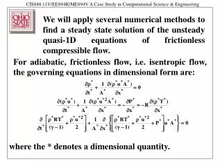
We will apply several numerical methods to find a steady state solution of the unsteady quasi-1D equations of frictionless compressible flow. For adiabatic, frictionless flow, i.e. isentropic flow, the governing equations in dimensional form are: where the * denotes a dimensional quantity.
Non-dimensionalize using: P = P*/Pref; Pref = 1 Lref = 1 cm. T = T*/Tref; Tref = 1 tref = Lref/uref r = r/rref; rref = Pref/Rtref = 1/R t = t*/tref u = u*/uref Non-dimensionalization of governing equations
Since tref = Lref/uref, this simply reduces to: Similarly, the momentum and energy equations reduce to: Non-dimensionalized governing equations
MacCormack’s explicit method Before proceeding with this numerical scheme, it is necessary to introduce artificial dissipation into each of the governing equations for stability:
Discretize the domain x [0,L] into N interior points and two boundary points labelled 0 and N+1, each spaced Dx apart: Next, the predictor and corrector parts of the algorithm are applied at each time step for each governing equation, at all interior points. MacCormack’s explicit method
One form for the artificial viscosity is as follows: for the predictor step, and for the corrector step. Coefficient of artificial viscosity • C=0.125 is a recommended value for this algorithm, for the non-dimensionalization shown in slide #2 of this lecture. • Note that there is nothing special about this value of 0.125 - you are encouraged to try different values as well as different expressions for ma and explore their effects on the final solution as well as on the convergence to the final steady state solution.
For obtaining supersonic solutions in the case study problem, you may prescribe any linearly decreasing pressure distribution p(x) from the inlet (say starting at a non-dimensional value of 1) to (say 0.015 at) the exit. Similarly, a linear profile can be prescribed for T(x) varying from 1 (non-dimensional) at the inlet to 0.2 at the exit. Linear for u(x) starting from 0.15 at inlet to 1.2 at exit. r(x) can be calculated from P(x)/T(x). None of these initial profiles are unique, but their judicious specification can accelerate the solution to the desired steady state solution. Initial Conditions
Inlet: Total pressure Po and Total temperature To are specified. Implicitly extrapolate for u(i=0): Determine T(i=0) from total temperature To and extrapolated value of u(i=0): Boundary Conditions
Before finding r(i=0), first find P(i=0) from assumption that flow is isentropic (i.e. loss-free) from supply to inlet, and from specification of Po and To: Boundary Conditions (contd.) • Now determine r(i=0) from:
Exit: To find supersonic solution, implicitly extrapolate for all computed variables: Boundary Conditions (contd.)
Pressure is determined from the equation of state: P(i=N+1) = r(i=N+1)T(i=N+1) Note that a supersonic steady state solution can also be obtained by prescribing a pressure at the exit plane that is low enough. What the exact value of this pressure would be cannot be determined a priori for more complicated problems. Specification of a Pexit that is higher than this value for supersonic flow results in the formation of standing normal shock waves in the diverging portion of the C-D nozzle. You are encouraged to experiment with these various boundary conditions in your homework assignments. Boundary Conditions (contd.)
Using Fourier stability analysis, it can be shown that this scheme is stable provided a(Dt)/(Dx) 1. The quantity a(Dt)/(Dx) is called the Courant number and a(Dt)/(Dx) 1 is called the Courant condition, where a is the relevant speed of sound in the problem. Courant condition
FTBS (Forward in Time, Backward in Space) Scheme Given equations of the form , we forward difference in time and backward difference in the spatial coordinate: This is valid for a > 0. For a < 0, a forward difference in space must be used. This FTBS scheme is also called an upwindscheme.
Discretize the domain as before with MacCormack’s method (slide#5). Next, apply FTBS to the non-dimensionalized equations, and add artificial dissipation to each equation: FTBS method applied to Quasi-1D flow
A form for the artificial viscosity is as follows: Coefficient of artificial viscosity • C ranging from 0.125 to 3 is recommended for this algorithm, for the non-dimensionalization shown in slide #2 of this lecture, and may be required to vary with spatial location as well. • Note that there is nothing special about this range of values for C - you are encouraged to try different values as well as different expressions for ma and explore their effects on the final solution as well as on the convergence to the final steady state solution.
As with the MacCormack scheme, a Fourier stability analysis shows that the Courant condition a(Dt)/(Dx) 1 must be satisfied for stable time-marching using the FTBS or first order upwind explicit scheme. Similar stability analysis for the FTCS (Forward in Time, Central differenced in Space) is alwaysunstable. The BTCS or Backward in Time, Central differenced in Space is unconditionallystable. Initial conditions are same as described in slide #11. Boundary conditions are same as described in slides #12-#15. Stability, ICs and BCs
There are problems involving multiple time scales, where stiffness of the set of equations forces you to take (Dt) smaller than the maximum (Dt) allowed by the Courant condition for explicit methods. This makes computational time immense, so that it is necessary to use implicit methods for such multi-time scale problems. Note that time steps in implicit methods are not strictly governed by the Courant condition.
Consider the initial value problem with y(0)=1. Suppose we apply a simple explicit method such as Euler’s Forward Method: The exact solution to this problem is of course Detour on Stiffness
Now suppose l=106 and tn=2.763x10⁻⁵ Suppose the error tolerance is desired to be and that we only have to satisfy provided we do not amplify the previous error e(tn).
But this means that Assuming this yn is only one component of a larger system, this is unacceptable because the step size for the rest of the equations is determined by the time scale of a component which has decreased by 12 orders of magnitude (from 1 to 10-12) and is probably of no further physical interest! Another way to view this is that 1/l is the time constant. The smaller the time constant, the smaller must be the time step just to maintain stability. Thus, for stiff equations, the step size depends almost entirely on the stability of the numerical method and not on the accuracy. This is best resolved by using implicit methods which are unconditionally stable.