Specification Error II
Specification Error II. Aims and Learning Objectives. By the end of this session students should be able to: Understand the causes and consequences of multicollinearity Analyse regression results for possible multicollinearity Understand the nature of endogeneity

Specification Error II
E N D
Presentation Transcript
Aims and Learning Objectives • By the end of this session students should be able to: • Understand the causes and consequences of • multicollinearity • Analyse regression results for possible • multicollinearity • Understand the nature of endogeneity • Analyse regression results for possible endogeneity
Introduction In this lecture we consider what happens when we violate Assumption 7: No exact collinearity or perfect multicollinearity among the explanatory variables and Assumption 3: Cov(Ui, X2i) = Cov(Ui, X3i)... =... Cov(Ui,Xki) = 0
What is Multicollinearity? The term “independent variable” means an explanatory variable is independent of of the error term, but not necessarily independent of other explanatory variables. Definitions Perfect Multicollinearity: exactlinear relationship between two or more explanatory variables Imperfect Multicollinearity: two or more explanatory variables are approximatelylinearly related
Example: Perfect Multicollinearity Suppose we want to estimate the following model: If there is an exact linear relationship between X2 and X3. For example, if Then we cannot estimate the individual partial regression coefficients
This is because substituting the last expression into the first we get: If we let
Example: Imperfect Multicollinearity Although perfect multicollinearity is theoretically possible, in practice imperfect multicollinearity is what we commonly observed. Typical examples of perfect multicollinearity are when the researcher makes a mistake (including the same variable twice or forgetting to omit a default category for a series of dummy variables)
Consequences of Multicollinearity OLS remains BLUE, however some adverse practical consequences: 1. No OLS output when multicollinearity is exact. 2. large standard errors and wide confidence intervals. 3. Estimators sensitive to deletion or addition of a few observations or “insignificant” variables. Estimators non-robust. 4. Estimators have the “wrong” sign
Detecting Multicollinearity No formal “tests” for multicollinearity 1. Few significant t-ratios but a high R2 and a collective significance of the variables 2. High pairwise correlation between the explanatory variables 3. Examination of partial correlations 4. Estimate auxiliary regressions 5. Estimate variance inflation factor (VIF)
Auxiliary Regressions Auxiliary Regressions - regress each explanatory variable on the remaining explanatory variables The R2 will show how strongly Xji is collinear with the other explanatory variables
Variance Inflation Factor In the two variable model (bivariate regression) the variance of the OLS estimator was: where Extending this to the case of more than two variables leads to the formulae laid out in lecture 5, or alternatively:
Example: Imperfect Multicollinearity CON INC WLTH 1 70 80 810 2 65 100 1009 3 90 120 1273 4 95 140 1425 5 110 160 1633 6 115 180 1876 7 120 200 2052 8 140 220 2201 9 155 240 2435 10 150 260 2686 Hypothetical data on weekly family consumption expenditure (CON), weekly family income (INC) and wealth (WLTH)
Regression Results: CON = 24.775 + 0.942INC -0.0424WLTH (3.669) (1.1442) (-0.526) (t-ratios in parentheses) R2 = 0.964 ESS = 8,565.554 RSS = 324.446 F= 92.349 R2 is high (96%); wealth has the wrong sign but neither slope coefficient is individually statistically significant. Joint hypothesis, however, is significant
Auxiliary Regression Results: INC = -0.386 + 0.098WLTH (-0.133) (62.04) (t-ratios in parentheses) R2 = 0.998 F= 3849 Variance Inflation Factor:
Remedying Multicollinearity High multicollinearity occurs because of a lack of adequate information in the sample 1. Collect more data with better information. 2. Perform robustness checks 3. If all else fails at least point out that the poor model performance might be due to the multicollinearity problem (or it might not).
The Nature of Endogenous Explanatory Variables • In real world applications we distinguish • between: • Exogenous (pre-determined) Variables • Endogenous (jointly determined) Variables When one or more explanatory variable is endogenous, there is implicitly a system of simultaneous equations
Example: Endogeneity But Therefore Cov(S, U) 0 OLS of the relationship between W and S gives “credit” to education for changes in the disturbances. Resulting OLS estimator is biased upwards (since Cov (Si, Ui) > 0) and, because the problem persists even in large samples, the estimator is also inconsistent
Remedies for Endogeneity • Two options: • Try and find a suitable proxy for the unobserved • variable • Leave the unobserved variable in the error term • but use an instrument for the endogenous • explanatory variable • (involves a different estimation technique)
Example and Include a proxy for ability Find an instrument for education Needs to have the following properties Cov(Z,U) = 0 and Cov(Z, S) 0
Hausman Test for Endogeneity Suppose we wish to test whether S is uncorrelated with U. Stage 1: Estimate the reduced form: Stage 2: Add to the structural equation and test the significance of Decision rule: if is significant reject null hypothesis of exogeneity
Summary In this lecture we have: 1. Outlined the theoretical and practical consequences of multicollinearity 2. Described a number of procedures for detecting the presence of multicollinearity 3. Outlined the basic consequences of endogeneity 4. Outlined a procedure for detecting the presence of endogeneity