Download
1 / 22
240 likes | 420 Views
O 9.1. 9. The Aggregate Expenditures Model. Chapter Objectives. Economists Combine Consumption and Investment to Depict an Aggregate Expenditures Schedule for a Private Closed Economy Three Characteristics of the Equilibrium Level of Real GDP in a Private Closed Economy AE = Output

E N D
O 9.1 9 The Aggregate Expenditures Model
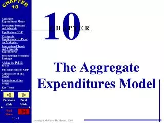
Chapter Objectives • Economists Combine Consumption and Investment to Depict an Aggregate Expenditures Schedule for a Private Closed Economy • Three Characteristics of the Equilibrium Level of Real GDP in a Private Closed Economy • AE = Output • Saving = Investment • No Unplanned Changes in Inventories • How Changes in Equilibrium Real GDP Occur and Relate to Multiplier • Integrate Government and Foreign Sectors into AE • Recessionary and Expansionary Expenditure Gaps
Consumption and Investment • Simplifications • Private Closed Economy • Planned Investment • Investment Schedule Investment Demand Curve Investment Schedule Investment Demand Curve Investment Schedule Ig 20 Investment (billions of dollars) r and i (percent) 8 20 20 ID 20 Investment (billions of dollars) Real GDP (billions of dollars)
W 9.1 Consumption and Investment • Equilibrium GDP: C + Ig = GDP • Real Domestic Output • Aggregate Expenditures • Aggregate Expenditures Schedule • Equilibrium GDP • Disequilibrium
(2) Real Domestic Output (and Income) (GDP=DI) (3) Con- sump- tion (C) (7) Unplanned Changes in Inventories (+ or -) (8) Tendency of Employment Output and Income (5) Investment (Ig) (6) Aggregate Expenditures (C+Ig) (1) Employ- ment (4) Saving (S) (1-2) Consumption and Investment …in Billions of Dollars • 40 • 45 • 50 • 55 • 60 • 65 • 70 • 75 • 80 • 85 $370 390 410 430 450 470 490 510 530 550 $375 390 405 420 435 450 465 480 495 510 $-5 0 5 10 15 20 25 30 35 40 20 20 20 20 20 20 20 20 20 20 $395 410 425 440 455 470 485 500 515 530 $-25 -20 -15 -10 -5 0 +5 +10 +15 +20 Increase Increase Increase Increase Increase Equilibrium Decrease Decrease Decrease Decrease Graphically…
530 510 490 470 450 430 410 390 370 Consumption (billions of dollars) 45° • 390 410 430 450 470 490 510 530 550 Disposable Income (billions of dollars) G 9.1 Consumption and Investment Equilibrium GDP C + Ig (C + Ig = GDP) C Equilibrium Point Aggregate Expenditures Ig = $20 Billion C = $450 Billion
Equilibrium GDP • Other Features… • Saving Equals Planned Investment • Leakage • Injection • No Unplanned Changes in Inventories
510 490 470 450 430 Aggregate Expenditures (billions of dollars) 45° 430 450 470 490 510 Real GDP (billions of dollars) Changes in Equilibrium GDP …and the Multiplier (C + Ig)1 (C + Ig)0 (C + Ig)2 Increase in Investment Decrease in Investment
International Trade • Net Exports and Aggregate Expenditures • Net Exports Schedule • Net Exports and Equilibrium GDP • Positive Net Exports • Negative Net Exports • International Economic Linkages • Prosperity Abroad • Tariffs • Exchange Rates
510 490 470 450 430 Aggregate Expenditures (billions of dollars) 45° 430 450 470 490 510 Real GDP (billions of dollars) +5 0 -5 Net Exports Xn (billions of Dollars) Real GDP International Trade Net Exports and Equilibrium GDP C + Ig+Xn1 C + Ig Aggregate Expenditures with Positive Net Exports C + Ig+Xn2 Aggregate Expenditures with Negative Net Exports Positive Net Exports Xn1 450 470 490 Xn2 Negative Net Exports
GLOBAL PERSPECTIVE -700 200 150 100 50 0 50 100 150 200 250 International Trade Net Exports of Goods - Select Nations, 2004 Negative Net Exports Positive Net Exports +37 Canada -17 France Germany +195 Italy -2 Japan +111 -117 United Kingdom -707 United States Source: World Trade Organization
(1) Level of Output and Income (GDP=DI) (5) Net Exports (Xn) (7) Aggregate Expenditures (C+Ig+Xn+G) (2)+(4)+(5)+(6) (2) Consump- tion (C) (4) Investment (Ig) (6) Government (G) Exports (X) Imports (M) (3) Saving (S) Adding the Public Sector Government Purchases and GDP …in Billions of Dollars • $370 • 390 • 410 • 430 • 450 • 470 • 490 • 510 • 530 • 550 $375 390 405 420 435 450 465 480 495 510 $-5 0 5 10 15 20 25 30 35 40 $20 20 20 20 20 20 20 20 20 20 10 10 10 10 10 10 10 10 10 10 10 10 10 10 10 10 10 10 10 10 20 20 20 20 20 20 20 20 20 20 $415 430 445 460 475 490 505 520 535 550
Aggregate Expenditures (billions of dollars) 45° 470 550 Real GDP (billions of dollars) Adding the Public Sector Government Spending and GDP C + Ig + Xn + G C + Ig + Xn C Government Spending of $20 Billion $20 Billion Increase in Government Spending Yields an $80 Billion Increase In GDP
Aggregate Expenditures (billions of dollars) 45° 490 550 Real GDP (billions of dollars) Adding the Public Sector Lump-Sum Tax Increase and GDP C + Ig + Xn + G Cd + Ig + Xn + G $15 Billion Decrease In Consumption From a $20 Billion (MPC=.75) Increase in Taxes $20 Billion Increase in Taxes Yields a $60 Billion Decrease In GDP
G 9.2 W 9.2 Adding the Public Sector Cd + Ig + Xn + G = GDP • Leakages • Injections • No Planned Inventory Changes Sd + M + T = Ig + X + G
550 530 510 490 470 Aggregate Expenditures (billions of dollars) 45° 490 510 530 Real GDP (billions of dollars) Equilibrium Versus Full-Employment GDP Recessionary Expenditure Gap AE0 $5 Billion Gap Yields $20 Billion GDP Change AE1 Recessionary Expenditure Gap = $5 Billion Full Employment
550 530 510 490 470 Aggregate Expenditures (billions of dollars) 45° 490 510 530 Real GDP (billions of dollars) Equilibrium Versus Full-Employment GDP Inflationary Expenditure Gap AE2 AE0 Inflationary Expenditure Gap = $5 Billion $5 Billion Gap Yields $20 Billion GDP Change Full Employment
W 9.3 Equilibrium Versus Full-Employment GDP • Application: • U.S. Recession of 2001 • Inflationary Expenditure Gap • U.S. Inflation in the Late 1980s • Full-Employment Output with Large Negative Net Exports • Negative Net Exports
Equilibrium Versus Full-Employment GDP • Limitations of the Model • Does Not Show Price Level Changes • Ignores Premature Demand-Pull Inflation • Limits Real GDP to the Full-Employment Level of Output • Does Not Deal with Cost-Push Inflation • Does Not Allow for “Self-Correction”
O 9.2 Say’s Law - The Great Depression and Keynes Last Word • Classical School – Automatic Self-Adjustment to Full Employment – Mill, Ricardo • Views Based Upon “Say’s Law” - J.B. Say (1767-1832) – Supply Creates its Own Demand • Great Depression Caused Questions • Keynes Answered in his General Theory of Employment, Interest, and Money • Income and Saving Discrepancies • Volatility in Investment Spending • Cyclical Unemployment Can Occur • Government Should Be Active in the Recovery Process
planned investment investment schedule aggregate expenditures schedule equilibrium GDP leakage injection unplanned changes in inventories net exports lump-sum tax recessionary-expenditure gap inflationary-expenditure gap Key Terms
Next Chapter Preview… Aggregate Demand and Aggregate Supply Chapter 10!