Topic 1(a): Review of Consumer Theory (demand)

1. Topic 1(a): Review of Consumer Theory (demand) Review of Demand. • Three areas to cover on the demand side: • Interpreting an individual consumer’s demand curve • Measuring consumer well-being using the demand curve • Deriving aggregate demand from individual demand

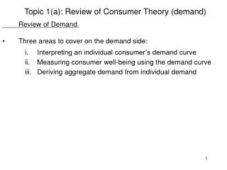
2. Topic 1(a): Review of Consumer Theory Demand curves usually slope downwards: known as the “law” of demand. • Interpreting an individual’s demand curve • Recall that a demand curve maps out a relationship between price and quantity. Price (P) Remember, on the horizontal axis we are measuring units of the good consumed (Q), Demand Curve (D) while on the vertical axis we are measuring the price per unit (P), in some form of currency (dollars, cents etc). Quantity (Q) How to interpret this demand curve? Two interpretations, each of which will be useful, depending on the context.

3. Topic 1(a): Review of Consumer Theory Interpretation 1: the D curve tells is how many units of a good a consumer wishes to buy in total, at a given price per unit for the good. P • The first interpretation of the demand curve is probably the most familiar to you: D For instance, the D curve tells us that if the price per unit is P1, then the consumer would like to buy Q1 units. P1 P2 etc. Q1 Q2 Q We can think of this interpretation as reading the D curve horizontally: that is, if we plug in values for P, we get out values for Q.

4. Topic 1(a): Review of Consumer Theory Interpretation 2: the height of the D curve at any given point tells is how the consumer values additional units of the good. P • The second interpretation of the demand curve may be less familiar to you: D For instance, the D curve tells us that if the consumer is currently has Q1 units of the good, then a small increase in quantity would be worth P1 per unit to the consumer. P1 P2 etc. Q1 Q2 Q We can think of this interpretation as reading the D curve vertically: that is, if we plug in values for Q, we get out values for P. We will elaborate on this interpretation by use of an example.

5. Topic 1(a): Review of Consumer Theory From the D function, if P=$10, Q=0 will be demanded. But if P = $8, Q = 1 will be demanded. P($) Example: Suppose that demand is given by Q = 5 - (1/2)P. 10  consumer’s maximum willingness to pay for the first unit is greater than $8, but less than $10. 8 Area of the rectangle ($10) thus gives an upper bound on consumer’s willingness to pay for the first unit. D Q 1 5 So we know that the maximum willingness to pay for the first unit is something greater than $8, but less than $10. Can we do better than this?

6. Topic 1(a): Review of Consumer Theory Consumer did not buy the first half unit when it cost $5, but does when it costs $4.50. P($) Now consider smaller changes in P. Say P from $10 to $9 so that Qfrom 0 to 0.5.  consumer’s maximum willingness to pay for this first half unit is something less than $5. 10 9 Now suppose P from $9 to $8, so that total Q from 0.5 to 1. 8 Consumer did not buy the second half unit when it cost $4.50, but does when it costs $4.00. D Q 5 1 0.5  consumer’s maximum willingness to pay for this second half unit is something less than $4.50. This tells us that the consumer’s maximum willingness to pay for the first unit is greater than $8, but in fact something less than $9.50 (as opposed to $10).

7. Topic 1(a): Review of Consumer Theory P($) We could consider even smaller changes in prices and quantities. In the limit, as we consider smaller and smaller price changes, what we are doing here is calculating the area under the demand curve between Q=0 and Q=1. 10 9 8 D Q 0.5 1 5 This area tells us the exact maximum willingness to pay by this consumer for the first unit of the good. In this case, the area of that trapezoid is equal to $9.  The consumer is willing to pay at most $9 for the first unit.

8. Topic 1(a): Review of Consumer Theory In this case, that area equals $7. P($) By the same logic, the area under the demand curve as we increase Q from 1 to 2 units tells us the maximum willingness to pay for the second unit. Indeed, the area under a D curve between any two quantities tells us the maximum willingness to pay for that additional quantity. 10 8 6 If we consider very small increases in quantity, than the trapezoid representing the willingness to pay has a very small base. Q 1 5 2 In the limit, as we consider tiny tiny increases in Q, the base of the trapezoid goes to zero, and the willingness to pay (per unit) for these tiny tiny increases in Q is just equal to the height of the demand curve.

9. Topic 1(a): Review of Consumer Theory As we have seen, this is equivalent to telling us how much the consumer is willing to pay for small Q. P($) This is the logic behind the second interpretation of the demand curve, that the height at any point tells us how consumers value small Q. 10 We can also think about this as telling us how much additional benefit a consumer would get from a small Q. 8 6 When we are thinking about the D curve in this way, we will refer to it variously as the: Q 2 Marginal Value (MV) curve Marginal Willingness to Pay (MWP) curve Marginal Benefit (MB) curve Note that these terms are equivalent!

10. Topic 1(a): Review of Consumer Theory 1st interpretation of D curve: tells us Q demanded at a given P. 2nd interpretation of D curve: area under the D curve measures consumer’s willingness to pay for Q1 units. P($) • Measuring consumer well-being using the demand curve. But, how much did consumer actually have to pay for Q1? A Expenditure (price times quantity) given by area P1Q1. P1  consumer willing to pay more than she has to pay. Difference between willingness to pay and expenditure measures consumer well-being. Q Q1 Definition: consumer surplus (CS) = what a consumer is willing to pay minus what they have to pay = NB from consuming that Q. In the diagram above, the CS from buying Q1 units at P1 per unit is equal to the triangle A.

11. Topic 1(a): Review of Consumer Theory Suppose two individuals - A and B - each with D curves drawn below. P P Aggregate D DB • Deriving aggregate demand from individual demand DA 3 1 QB QA 4 2 5 3 9 5 At $3, A demands 2 and B demands 3. Aggregate demand at $3therefore equals 2+ 3 = 5. At $1, A demands 4, B demands 5, and agg. D = 4+5=9. We are horizontally aggregating individual demands to get aggregate demand.