Looking at Data-Distributions
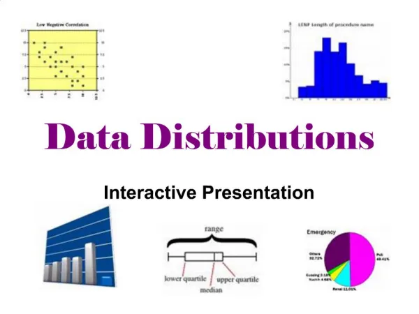
This guide provides a comprehensive overview of data distributions, emphasizing the importance of context in interpreting numerical values. It covers key concepts such as individuals, variables (categorical and quantitative), and how to represent data visually using pie charts, bar graphs, and histograms. The text illustrates various concepts through examples, including a back-to-back stem plot for comparing study times between genders. Additionally, it delves into measures of center (mean and median) and spread (quartiles, IQR, and standard deviation), highlighting the significance of understanding variability when analyzing data.

Looking at Data-Distributions
E N D
Presentation Transcript
Looking at Data-Distributions 1.1-Displaying Distributions with Graphs
Basic definitions • Data-numbers with a context • Eg. Your friends new baby weighed 10.5 pounds, we know that baby is quite large. But if it is 10.5ounces or 10.5kg, we know that it is impossible-the context makes the number informative • Individuals-objects described in the data(people,animals,things) • Variable-any property/characteristics of an individual(IQ scores of persons) • Distribution-of a variable tells us what values & how often(frequency of a variable)
Types of variables • categorical variable-places an individual into one of several categories(male/female, smoker/nonsmoker) • quantitative variable-takes numerical values for which arithmetic operations such as adding & averaging can be performed(shoe size,age)
How to represent data? • Categorical variables-can use Pie-chart & bar graphs • Eg. make a pie chart/bar graph for distribution of gender • Quantitative variables-can use histogram
Example 1-The color of your car(distribution of the most popular colors for 2005 model luxury cars made in North America • What percent of vehicles are some other color? • Make a bar graph? • Can we make a pie chart for the given colors? • Would it be correct to make a pie chart if you added an “Other” category?
Example 2-The density of the earth (the variable recorded was the density of the earth as multiple of the density of water)
Using TI-84 create a histogram • Discuss the shape, center, spread and outliers
Example3-Do women study more than men?Variable-minutes studied on a typical weeknight of a first-year college class • Here are the responses of random samples of 30 women and 30 men from the class: • Women 180,120,150,200,120,90,120,180,120,150,60,240,180,120,180,180,120, 180,360,240,180,150,180,115,240,170,150,180,180,120 • Men 90,90,150,240,30,0,120,45,120,60,230,200,30,30,60, 120, 120, 120, 90,120,240,60,95,120,200,75,300,30,150,180 • Examine the data. Why are you not surprised that more responses are multiples of 10minutes? We eliminated one student who claimed to study 30,000 minutes per night. Are there any other responses you consider suspicious? • Make a back-to-back stem plot to compare the two samples. That is, use one set of stems with two sets of leaves, one to the right and one to the left of the stems.(Draw a line on either side of the stems to separate stems and leaves.) Order both sets of leaves from smallest at the stem to largest away from the stem. Report the approximate midpoints of both graphs. Does it appear that women study more than men(or at least claim that they do)?
Answers • a) Most people round their answers. The students who claimed 0 minutes, 360 minutes and 300 minutes. • B)The stemplots suggest that women(claim to) study more than men. The approximate centers are 175 minutes for women and 120 minutes for men.
Looking at Data-Distributions 1.2-Describing Distributions with numbers
Mean & Median • Mean =sum of numbers/ number of numbers • Median=Middle value(when the numbers are in ascending order) • Example 1: 103,105,109,140,170 (Median is 109-the number in the (n+1)/2th position from the bottom of the list-n is number of values) • Example 2: 18,19,20,20,26,28(Median is 20- the avg of n/2 position number & n/2+1 position). Mean =21.83 • Example 3: replace 28 in example 2 by 100 & re -compute mean and median? • 18,19,20,20,26,100 • Mean =33.83 • Median-does not change Mean is affected by outliers Median is not affected by outliers A measure of center alone can be misleading Solution-need a measure of spread(variability)
Measuring spread Quartiles • Example 4–Age of 10 students • 26,19,20,18,20,19,19,19,19,21 • Sort them in ascending order • 18,19,19,19,19,19,20,20,21,26 • Median =19 (Q2 ) • First quartile=median of the lower half of data(Q1 )=19 • Third quartile=median of the upper half of data(Q3 )=20
Five-number summary • Min Q1 Q2 Q3 Max • Box plot- Picture of the five number summary. Can be used to compare two distributions • IQR(Inter quartile range)= Q3 - Q1 Max Q3 IQR Median(Q2 ) Q1 Min
The 1.5 X IQR rule for suspected outliers • Example 5(travel times to work in New York-in minutes) • 10,30,5,25,40,20,10,15,30,20,15,20,85,15,65,15,60,60,40,45 • (single peaked/right skewed/no center observation,but there is a center pair) • The five number summary • 5 15 22.5 42.5 85 • IQR=42.5-15=27.5 • Apply 1.5XIQR rule • Step 1:calculate 1.5 X IQR=1.5 x 27.5 • Step 2: Calculate Q1 -(1.5 X IQR)= 15-41.25=-26.25 • Step 3: Calculate Q3 +(1.5 X IQR)=42.5+41.25=83.75 • Any values outside of (-26.25,83.75) are flagged as outliers • The suspected outlier in the data is 85
Standard deviation(s) • Used as a measure of spread when mean=center • Units of s=same as data units • s always positive • Higher s->more spread • s=0->no spread -> all observations equal • s affected by outliers • Example :1,1,2,5,3
Looking at Data-Distributions 1.3 –Density Curves and Normal Distributions
Definitions • Density Curve-Special type of histogram such that total area under the curve is 1 • Typical histogram • Example for a Density Curve Relative frequency Bin limits • Characteristics of density curve • All y values positive • total area under curve=1 • Curve approaches to zero for extreme left & right x values
Definitions Normal Distribution • Formula It can be shown that the probability density function for a normal random variable, X, with mean X and standard deviation X has the following form. • TI-84 calculator-> 1)STAT plot off 2) enter in Y1-use normalpdf(x,mean,standard deviation) 3)normalpdf( ) found in 2nd->DISTR
Definitions The 68-95-99.7 rule • Example-When Mean 0 & standard deviation is 1 • Approximately 68% of the observations fall within one standard deviation of the mean • Approximately 95% of the observations fall within two standard deviation of the mean • Approximately 99.7% of the observations fall within three standard deviation of the mean
Definitions • tables-allows us to calculate the probabilities for a normal distribution • How to get numbers? • There are too many normals(one per possible mean/one per possible standard deviation) • >infinitely many • Need to standardize • Standardization of Normal Random Variables. If X is normally distributed, its standardization is • Equation:
Definitions • Standard normal(Z) : N(0,1) , mean 0 & Standard deviation 1 • Now can calculate the fraction of my data set between any two limits