Understanding Productivity, Output, and Employment in Economic Analysis
This lecture explores the relationship between productivity, output, and employment within an economy. It highlights key factors determining labor supply and demand, equilibrium in the labor market, and overall output generated. Using the Cobb-Douglas production function as a framework, we examine how inputs like capital and labor impact productivity. The discussion includes real-world examples, such as the impact of capital on productivity within industries, and explores the concept of marginal productivity. Additionally, we address how changes in the production function can signify supply or productivity shocks in the economy.


Understanding Productivity, Output, and Employment in Economic Analysis
E N D
Presentation Transcript
How much does the economy produce? • The quantity that an economy will produce depends on two things- • The quantity of inputs utilized in the production process and • The PRODUCTIVITY of the inputs • An economy’s productivity is basic to determining living standards. • In this lecture we shall see how productivity affects people’s incomes by helping to determine how many workers are employed and how much they receive. • Among all the inputs for production, labor is usually considered the most important input. • Therefore, first we shall study the factors that determine demand and supply of labor and then the forces that bring the labor market into equilibrium. • Equilibrium in the labor market determines wages and employment; and the level of employment together with other inputs and the level of productivity determines how much output en economy produces.
The production function • The quantity of inputs does not completely determine the amount of output produced. • How effectively the factors of production are used is also important. • The effectiveness with which factors of production are used may be expressed by a relationship called the production function. • Mathematically, we express production function as- Y = A f(K, N, L, …) • Where, Y stands for output, A stands for a number that indicated productivity, K stands for capital, N stands for number of labor employed, L stands for land. Other factors could be, machinery, energy, building etc. • The symbol “A” in the equation above captures the overall effectiveness of the factors of production. We call A the “total factor productivity”.
Empirical example: US production function • Studies show that the relationship between outputs and inputs in the US economy is described reasonably well by the following production function: • This type of production function is called the Cobb-Douglas production function. • Historical GDP data of US for the period 1899 – 1922 showed that the production function for US followed the form:
Shape of the production function • We can have an idea about the shape of the production function by holding one of the two factors of production and the value of total factor productivity (A) constant. • For example, if we want to see the relationship between capital and total output for the year 2001, then we hold the values of A and N constant for that year and treat K as variable. • As a result our production function gets the shape as:
Shape of the production function: Properties • The production function slopes upward from left to right: this means that as the capital stock increases more output can be produced. • The slope of the production function becomes flatter from left to right: this means that although more capital always leads to more output, it does so at a decreasing rate.
Effect of increasing 1000 units of capital each time Marginal Product of Capital: Marginal product of capital between K = 2000 and 3000 What is the marginal product of capital between K = 4000 and 5000? Is it less than the previous one? What does it mean?
Marginal productivity • The previous example shows that marginal productivity is falling as we increase the amount of capital • Generally, when amount of labor is high compared to the amount of capital, marginal productivity of capital is high. Alternatively, when amount of labor is low compared to the amount of capital, marginal productivity of labor is high • Real life example: Adamjee Jute Mill had many workers employed against every single machine. Therefore, productivity of workers were low as many workers used to sit idle without a machine to work with. If we would have increased number of machines, perhaps, we could have increased production of jute; and as a result productivity of workers would have increased. Unfortunately, we shut down the mill!!!!
Formal Definitions of Marginal Productivity • Marginal Productivity of Capital: means additional output produced by each additional unit of capital. • Marginal Productivity of Labor: means additional output produced by each additional unit of labor. • Because of diminishing marginal productivity for both labor and capital the slope of production function becomes flatter from left to right. • If the marginal productivity were increasing, slope of the production function would become steeper from left to right. • If the marginal productivity were constant, the slope would be constant and the shape of the curve of production function would be a straight line.
Changes in the production function • The production function does not remain fixed over time. It may change. • Economists use the term “supply shock” or “productivity shock” to refer to change in an economy’s production function. • A positive supply shock raises the amount of output, and a negative supply shock reduces the amount of output. • Sources of supply shock: natural calamities, changes in govt. regulation, innovations etc. Y Production function before the shock Production function after the shock Factor of production
Demand for labor • In contrast to the amount of capital, the amount of labor employed in the economy can change quickly. • Thus, year-to-year changes in production can be traced to the changes in employment. • Demand for labor determines the level of employment. • For this reason, understanding demand for labor is important. • To understand demand for labor we shall make the following assumptions to keep things simple: • Workers are alike • Firms have to pay competitive wage to hire workers • Firms objective is to maximize profit
Determination of the demand for labor • Demand for labor is determined based on the marginal product of labor, cost of labor and price of the product that labor produces. • Example: Suppose, wage rate of labor is Tk. 80/day.
Determination of demand for labor • To maximize profit the firm will follow the following rules: The expression “W/price” is called, in economics, “real wage”. Why? Because when we divide wage by price we get a figure that shows the units of physical goods produced by labor.
Determination of labor demand The MPN curve on the right can be thought of as the demand for labor. Because quantity of labor is determined by the price of labor (the real wage). What happens when the MPN > w*? Firms hire more labor. What happens when MPN < w*? Firms lay-off labor What happens at point A? Equilibrium established. MPN and real wage A Real wage w* MPN N* labor
Factors that shift labor demand curve • Changes in the wage do not shift the labor demand curve. Changes in the wage will cause movement along the labor demand curve. • Factors that shift labor demand curve would be something that will change the demand for labor at any given wage. • A beneficial shock will shift the labor demand curve to the right. • An adverse shock will shift the labor demand curve to the left.
Shift of the labor demand curve • A beneficial supply shock, such as invention of a new technology, will shift the MPN curve to the right. • Originally, the firm employed N* amount of labor. • Now the real wage and the new MPN curve intersects at point C up to which the firm will want to hire labor to maximize profit. • As a result employment will rise and new employment level will be at X. MPN and real wage B A C Real wage w* MPN 2 MPN 1 N* X labor
Supply of labor • We have seen that firm’s demand for labor depend on labor productivity and wage paid to labor. • However, supply of labor depends on workers’ personal choice to work. • Personal choice about being a part of the labor force generally depends on the following two factors: • Income-leisure trade-off • Real wage
Labor supply curve • Labor supply curve looks the same as the supply curve we studied before. • Usually, we assume that a higher real wage will increase labor supply. • Labor supply curve will not shift because of a change in the wage. • Any factor that changes the amount of labor supply at a given wage rate will shift the labor supply curve.
Labor market equilibrium MPN and real wage Labor supply A Real wage w* MPN/demand for labor labor
When profit maximizing wage is higher than equilibrium wage • Labor market equilibrium is at point A. • But, as the profit maximizing wage is higher than the equilibrium wage, firms will hire labor that corresponds to point C, where N1 amount of labor is employed by the firms. • As a result, although the potential labor supply will be at point B, N2 amount of labor will not be employed. • This gives the firm the power to lower wage until equilibrium is reached at point A. MPN and real wage Labor supply C B w’ Profit max wage A w* equilibrium wage MPN/demand for labor N1 N* N2 labor
Effects of adverse supply shock real wage 1. A temporary adverse supply shock NS 2. Real wage falls A w2 B w1 ND 1 ND2 labor N2 N1 2. Employment falls
What if all workers are not alike? • We assumed that all workers are alike. By this, we meant that all workers have the same skill level. • However, if workers have different skill level then supply shocks will not affect all workers in the same way. • Example: if a production process introduces computer based production, then workers who can operate computers will cope with the new process quickly. On the other hand, workers who cannot operate computers will find it difficult to cope with the process. This will create difference in the marginal productivity level of these two groups of workers. Most likely, the workers who can use computers will get higher wage at cost of those who cannot. • Therefore, whether a shock will be considered beneficial or adverse depends on the skill/education level of the workers.
Unemployment: the untold story of full-employment • Full-employment level implies that all the workers who are willing to work at the equilibrium wage rate will find a job. • All workers in real life do not find jobs even if they want to. When workers are unemployed for a long time the sum of all such workers constitute “structural unemployment”. • If workers are unemployed for a brief period (for example: the brief period in which they search for a suitable job) we call it “frictional unemployment”. • The rate of unemployment that prevails when output and unemployment r ate the full-employment level, we call it natural rate of unemployment. • The difference between actual unemployment rate and natural unemployment rate is called cyclical unemployment. • If workers are not willing to work, this will not constitute unemployment. We shall consider these workers as out of work force.