Vulnerability and Adaptation Assessment Hands-on Training Workshop Climate Change Scenarios

1. Vulnerability and Adaptation Assessment Hands-on Training WorkshopClimate Change Scenarios

2. Outline • Brief review of climate change • Why we use scenarios • Review of options • Incremental • Analogue • Models • GCMs • Use of GCMs • Downscaling options • Statistical downscaling • RCMs

3. Outline (continued) • Techniques for understanding the range of regional climate change • What to use under what conditions • Obtaining data

4. Brief Primer on RegionalClimate Change • Temperatures over most land areas are likely to rise • Other factors, e.g., land use change, may also be important • Warmer temperatures mean increases in heat waves and evaporation • Global-mean sea level rise: 0.1 to 0.9 m • Modified by local subsidence/uplift • Precipitation will change; increase globally • Local changes uncertain: critical uncertainty • Increase in storm intensity in some regions

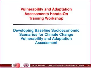
5. Normalized Annual-Mean Temperature Changes in CMIP2 Greenhouse Warming Experiments

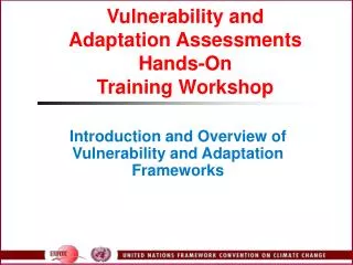
6. -6 0 6 -9 -3 3 9 Normalized Annual-Mean Precipitation Changes in CMIP2 Greenhouse Warming Experiments %

7. Why Use Climate Change Scenarios? • We are unsure exactly how regional climate will change • Scenarios are plausible combinations of variables consistent with what we know about human-induced climate change • One can think of them as the prediction of a model, contingent upon the GHG emissions scenario • Since estimates of regional change by models differ substantially, an individual model estimate should be treated more as a scenario

8. What Are Reasonable Scenarios? • Scenarios should be: • Consistent with our understanding of the anthropogenic effects on climate • Internally consistent • e.g., clouds, temperature, precipitation • Scenarios are a communication tool about what is known and not known about climate change • Should reflect plausible range for key variables

9. Scenarios for Impacts Analysis • Need to be at a scale necessary for analysis • Spatial • e.g., to watershed or farm level • Temporal • Monthly • Daily • Sub-daily

10. Options for Creating Scenarios • Past climates: analogues • Spatial analogues • Arbitrary changes; incremental • Climate models

11. Past Climates • Options • Instrumental record • Paleoclimate reconstructions • Instrumental record • Pros • Can provide daily data • Includes past extreme events • Cons • Range of change in past climate is limited • Data can be limited

12. Past Climates (continued) • Paleoclimate reconstructions • From tree rings, boreholes, ice cores, etc. • Can give annual, sometimes seasonal, climate • Can go back hundreds of years • Pro • Wider range of climates • Cons • Incomplete data • Uncertainties about values

13. Mann et al. Reconstruction of N. Hemisphere Temperatures

14. Spatial Analogues

15. Spatial Analogues (continued) • Advantage • Communication tool: perhaps easier to understand • Disadvantages • Require using a model result to choose the spatial analogue region • Do not capture changes in variability

16. Arbitrary/Incremental Scenarios • Assume uniform annual or seasonal changes across a region • e.g., +2°C or +4°C for temperature • +/-10% or 20% change in precipitation • Can also make assumptions about changes in variability and extremes

17. Arbitrary/Incremental Scenarios (continued) • Pros • Easy to use • Can simulate a wide range of conditions • Cons • Assuming a uniform change over the year or across a region may fail to capture important seasonal or spatial details • Combinations of changes in climate for different variables can be physically implausible

18. Climate Models • Models are mathematical representations of the climate system • They can be run with different forcings, e.g., higher GHG concentrations • Models are the only way to capture the complexities of increased GHG concentrations

19. General Circulation Models • Pros • Can represent the spatial details of future climate conditions for all variables • Can maintain internal consistency • Cons • Relatively low spatial resolution • May not accurately represent climate parameters

20. Example of GCM Output

21. Downscaling from GCMs • Downscaling is a way to obtain higher spatial resolution output based on GCMs • Options include: • Combine low-resolution monthly GCM output with high-resolution observations • Use statistical downscaling • Easier to apply • Assumes fixed relationships across spatial scales • Use regional climate models (RCMs) • High resolution • Capture more complexity • Limited applications • Computationally very demanding

22. Combine Monthly GCM Output with Observations • An approach that has been used in many studies • Typically, one adds the (low resolution) average monthly change from a GCM to an observed (high resolution) present-day “baseline” climate • 30 year averages should be used, if possible • e.g., 1961-1990 or 1971-2000 • Make sure the baseline from the GCM (i.e., the period from which changes are measured) is consistent with the choice of observational baseline

23. Combining Monthly GCMs and Observations • This method can provide daily data at the resolution of weather observation stations • Assumes uniform changes within a GCM grid box and over a month • No spatial or daily/weekly variability

24. How Many GCM Grid Boxes Should Be Used • Using the single grid box that includes the area being examined would be ideal, but • There can be model noise at the scale of single grid boxes • Many scientists do not think single box results are reliable • Hewitson (2003) recommends using 9 grid boxes: the grid being examined plus the 8 surrounding grid boxes • Need to consider the total area covered by all those grid boxes. Does it include topography or climates not similar to the area being studied?

25. Statistical Downscaling • Statistical downscaling is a mathematical procedure that relates changes at the large spatial scale that GCMs simulate to a much finer scale • For example, a statistical relationship can be created between variables simulated by GCMs such as air, sea surface temperature, and precipitation at the GCM scale (predictors) with temperature and precipitation at a particular location (predictands)

26. Statistical Downscaling (continued) • Is most appropriate for • Subgrid scales (small islands, point processes, etc.) • Complex/heterogeneous environments • Extreme events • Exotic predictands • Transient change/ensembles • Is not appropriate for • Data-poor regions • Where relationships between predictors and predictands may change • Statistical downscaling is much easier to apply than regional climate modeling

27. Statistical Downscaling (continued) • Statistical downscaling assumes that the relationship between the predictors and the predictands remains the same • Those relationships could change • In such cases, using regional climate models may be more appropriate

28. Statistical Downscaling Model (SDSM) • Currently, only feasible based on outputs from a few GCMs

29. Global Data to Use in Downscaling with SDSM • Canadian site • Go to scenarios, then SDSM • Only has HadCM3 • Get output for individual grid

30. Regional Climate Models (RCMs) • These are high resolution models that are “nested” within GCMs • A common grid resolution is 50 km • Some are higher resolution • RCMs are run with boundary conditions from GCMs • They give much higher resolution output than CCMs • Hence, much greater sensitivity to smaller scale factors such as mountains, lakes

31. RCM Limitations • Can correct for some, but not all, errors in GCMs • Typically applied to one GCM or only a few GCMs • In many applications, just run for a simulated decade, e.g., 2040s • Still need to parameterize many processes • May need further downscaling for some applications

32. GCM vs. RCM Resolution Precipitation Temperature GCM RCM

33. Extreme Precipitation (JJA) RCM Observation GCM

34. By Now You May Be Confused • So many choices, what to do? • First, let’s remember the basics • Scenarios are essentially educational tools to help: • See ranges of potential climate change • Provide tools for better understanding the sensitivities of affected systems • So, we need to select scenarios that enable us to meet these goals

35. Tools for Assessing Regional Model Output • It is useful first to compare results from a number of GCMs that might be used to drive an RCM • Normalized GCM results allow comparison of the relative regional changes • Can analyze the degree to which models agree about change in direction and relative magnitude • A measure of GCM uncertainty

36. Tools for Assessing Regional Model Output (continued) • Agreement between GCMs does not necessarily mean that they are all correct – they may all be repeating the same mistakes • Still, GCMs are the primary tool for estimating the range of future possibilities

37. Normalizing GCM Output • Expresses regional change relative to an increase of 1°C in mean global temperature • This is a way to avoid high sensitivity models dominating results • It allows us to compare GCM output based on relative regional change • Normalized temperature change = ΔTRGCM/ΔTGMTGCM • Normalized precipitation change = ΔPRGCM/ΔTGMTGCM

38. Pattern Scaling • Is a technique for estimating change in regional climate using normalized patterns of change and changes in GMT • Pattern scaled temperature change: • ΔTRΔGMT = (ΔTRGCM/ΔTGMTGCM) x ΔGMT • Pattern scaled precipitation • ΔPRΔGMT = (ΔPRGCM/ΔTGMTGCM) x ΔGMT

39. Tools to Survey GCM Results • Finnish report: “Future climate . . .” • COSMIC • MAGICC/SCENGEN

40. Finnish Publication • Shows regional output on temperature and precipitation for a number of models • For three time slices over 21st century • Uses some scaling • Useful as a look-up to see degree of model agreement or disagreement • MAGICC/SCENGEN and COSMIC provide more flexibility to users

41. Finnish Environment Example

42. COSMIC • Developed by M. Schlesinger, R. Mendelsohn, and L. Williams • Can choose from 28 emission scenarios • Select individual GCM model • Results scaled • Select country • Area or population weighted • Yields annual change in GHGs, SO2, SLR, and temperature

43. COSMIC Output • Will give global changes in CO2, SO4, temperature, and sea level rise • Will also give month-by-month temperature and precipitation at the country level • Easy to use and obtain data • Analyst should not use raw output, but compute changes in temperature and precipitation

44. COSMIC Limitations • Since results are scaled, change will be smooth and will not reflect interannual variability • Since results are smoothed, it is sufficient to use a single year output as representative of average climate change • GCMs tend to be older than in SCENGEN • Are 2 x CO2; not transients • Does not have mapping capabilities of SCENGEN

45. MAGICC/SCENGEN • MAGICC is a simple model of global T and SLR • Used in IPCC TAR • SCENGEN uses pattern scaling for 17 GCMs • Yield • Model by model changes • Mean change • Intermodel SD • Interannual variability changes • Current and future climate on 5 x 5°grid

46. Using MAGICC/SCENGEN

47. MAGICC: Selecting Scenarios

48. MAGICC: Selecting Scenarios (continued)

49. MAGICC: Selecting Forcings

50. MAGICC: Displaying Results