Two points on the landscape

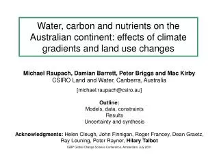
1. Water, carbon and nutrients on the Australian continent: effects of climate gradients and land use changes • Michael Raupach, Damian Barrett, Peter Briggs and Mac KirbyCSIRO Land and Water, Canberra, Australia • [michael.raupach@csiro.au] • Outline: • Models, data, constraints • Results • Uncertainty and synthesis • Acknowledgments: Helen Cleugh, John Finnigan, Roger Francey, Dean Graetz, Ray Leuning, Peter Rayner, Hilary Talbot • IGBP Global Change Science Conference, Amsterdam, July 2001

2. Two points on the landscape Savannah woodland Rainfall 800 mm Old-growth forest Rainfall 600 mm

3. ATMOSPHERE CO2 H2O N2, N2O Photosynthesis Rain WaterCycle N fixation,N deposition,N volatilisation C Cycle Transpiration PLANTLeaves, Wood, Roots Product offtake Respiration Fertiliser inputs N,P Cycles ORGANIC MATTER Litter: Leafy, Woody Soil: Active (microbial) Slow (humic) Passive (inert) SOIL Soil water Mineral N, P Sediment transport Runoff Leaching Water flow Linked terrestrial cyclesof water, C, N and P C flow N flow P flow

4. Modelling water, carbon and nutrient cyclesFramework: the dynamical system • Variables: X = {Xr} = set of stores (r) including all water, C, N, P, … stores F = {Frs} = set of fluxes (affecting store r by process s)M = set of forcing climate and surface forcing variablesP = set of process parameters • Stores obey mass balances (conservation equations) of form (for store r) • Statistical steady state or quasi-equilibrium solutions: • Fluxes are described by scale-dependent phenomenological equations of form Used here! Problem: find these for large scales!

5. Scaling: a general viewStatistical averaging of phenomenological equations • Requirement for scale consistency: • X, F, M and P are all defined with the same space and time averaging • Related to smaller-scale process descriptions by statistical averaging • Statistical averaging process: space or time averages of fluxes are Coarse-scale average flux Fine-scale model PDF of (X,M,P) = V Fine-scale model with coarse data Bias = [(co)variance] * [second derivative of Frs(V) ]

6. Evaporation and TranspirationSimplifying infiltration models to 2-layer soil, daily time step (Mac Kirby) Rain > Ksat2 Rain > Ksat1 Duplex soil Ksat1 >> Ksat2 Rain < Ksat 2 looks like clay

7. Evaporation and TranspirationA simple statistical-steady-state model • Evaporation is determined by (rainfall, energy) in (dry, wet) environments • [Energy-limited Evaporation] = [Priestley-Taylor Evaporation] = constant * [Available Energy] • A single-parameter hyperbolic function interpolates between dry and wet limits • [Total Evaporation] = [Plant Transpiration] + [Soil Evaporation] • Time average of [Soil Evaporation] / [Total Evaporation] = exp(-c*LAI) • Annual mean, catchment-scale water balance:

8. Evaporation and TranspirationTests of statistical-steady-state model • Annual mean, catchment-scale water balance

9. Evaporation and energy: forest sytemsRay Leuning and Helen Cleugh (CLW), Tumbarumba flux site • Daytime evaporation = 1.1 * equilibrium evaporation

10. Evaporation and energy: cropping sytemsChris J Smith and Frank Dunin, CSU Site, Wagga 60 Triticale, 1999 Lysimeters Priestley Taylor 50 40 30 20 10 0 Jul-99 Jan-00 Mar-99 Nov-99 May-99 Sep-99 Evapotranspiration (mm/week) 60 Lupin, 2000 50 40 30 20 10 0 Jul-00 Jan-01 Mar-00 Nov-00 Sep-00 May-00

11. Quasi-steady surface energy balance in an entraining convective boundary layer • Why Priestley-Taylor evaporation is a good measure of potential evaporation over a moist region parameter = relative deficit of entrained air

12. Net Primary Productivity (NPP) • [NPP] = [Photosynthetic Assimilation] - [Autotrophic Respiration] • A simple, linearised model for light and water limited NPP:

13. Testing predictions of NPPVast dataset (Barrett 2001) linear axes logarithmic axes

14. Testing predictions of NPPVast dataset (Barrett 2001) • NPP depends on saturation deficit, through water use efficiency MeasurementsModel

15. Biomass Litter C Soil C Bios Vast Testing predictions of C storesVast dataset (Barrett 2001)

16. Data requirements • Climate • Rainfall; solar irradiance; temperature; humidity • Land cover and land use • Vegetation properties (leaf area index; height) • Land use (forest / rangeland / crop / pasture / horticulture) • Land management • Fertiliser application rate (N, P) • N fixation by legumes • Irrigation • Soils • Soil type (via pedotransfer functions) => • Soil depth; soil texture; hydraulic properties; bulk density

17. C, N and P balances with present climate and agricultural nutrient inputsNet Primary Production • NPP broadly follows rainfall, with additional modulation by saturation deficit (through water use efficiency). Hence there is less NPP per unit rainfall in north than in south.

18. Effect of agricultureExample: ratio of (NPP with agriculture) / (NPP without agriculture) • NPP has increased locally (at scale of 5 km cells) by up to a factor of 2 in response to the nutrient inputs associated with European-style agriculture • Largest regional-scale increases occur in the WA, SA, Victorian and NSW wheatbelts

19. Mineral N balance Without agriculture • IN: fixation, small deposition • OUT: leaching, volatilisation, disturbance With agriculture • More fixation (x 2) • More disturbance

20. Summary • A formal dynamical-system framework • rigorous treatment of scaling, uncertainty, synthesis • Information flow: evaporation -> NPP -> fluxes and stores of C,N,P • Effects of agriculture on NPP, nitrogen and phosphorus: • Agricultural nutrient inputs (fertiliser, legumes) have led to regional-scale increases (relative to pre-agricultural conditions) of up to factor of 2 for NPP, and up to a factor of 5 for mineral N, labile P • Largest changes in N balance are fixation (sown legumes) and disturbance (herbivory) • Continental aggregates: • Mean continental NPP without agriculture is 0.96 GtC/year • Continental changes induced by agriculture: NPP + 4.8% mineral N + 13% labile P + 7.6% N budget (in, out) + factor 2

21. SynthesisA multiple-constraint approach (1) • Problem: What is the space-time distribution of the sources and sinks of CO2 (water, CH4, N2O, dust …) across a large region? • Available information from observations: • C(i) atmospheric concentrations: provide budget constraint • E(j) eddy fluxes: provide accurate point checks • R(k) remotely sensed data: provide indirect continental coverage • S(m) carbon stocks: provide biological linkage • Model: • Includes a (small) set of N parameters p which are poorly known • Predicts flux distribution F with given parameters p • Can also predict observable quantities (C, E, R, S) • How can we use observations (of C, E, R, S) to constrain p?

22. SynthesisA multiple-constraint approach (2) • Approach: • Use the model to predict the observed quantities C, E, R and S, and also the regional flux distribution F(p), using a consistent small set of parameters p • Determine p by minimising a multiple objective function JmultJmult = sum of several single objective functions (each a sum-of-squared errors) • Use p to determine regional flux distribution F(p) • Keys to approach: • Multiple (not necessarily direct) observations • A model which predicts F and all observables with common parameters p • Consistency check: use single objective functions (for C, E, R, S) separately