Download
1 / 30
300 likes | 315 Views
Explore the distribution of extreme waves using numerical modeling, focusing on wave scales, computational efficiency, and wave characteristics. Analyze the spectral development and probability distributions of wave heights. Investigate the unique Draupner wave event in the North Sea. Compare linear and non-linear wave theories for extreme events.

E N D
Distribution of extreme waves by simulation. • Herve’ Socquet-Juglard UiB (Bergen) • Kristian Dysthe ” • Karsten Trulsen UiO (Oslo) • Harald Krogstad NTNU (Trondheim) • Jingdong Liu ” Sponsors: The Research Council of Norway, Statoil and Hydro.
Length scales and computaional efficiency. • Scales in the range 10-3 -102 meters exist on the ocean surface • Most of the energy, however, is usually found in a rather narrow spectral range. • Our wave model, exploiting this fact is very efficient.
The computational domain. The efficiency of the numerical model permits a large artificial ”ocean” containing app. 10.000 waves at any given time. For comparison: a 20 min. wave record from a point observation contains 100-150 waves. 128 L 128 L L : typical wavelength
Truncated JONSWAP-spectrum Truncated at f = fp for different ”peak enhancements” gamma. Contains more than 80% of the spectral- energy.
Steepness: • Scatter-diagram of peak period Tp and significant wave height Hs . Data from the northern North Sea collected from 5 platforms 1973-2001. (Haver, Eik)
Spectral developmentbroad- and medium angular distribution(BFI=1.2)
”The Draupner wave” • 1st of January 1995 this wave was measured at the Draupner plattform in the North Sea. • The wave crest was 18.5 meters above the equilibrium surface. That is more than 6 times the standard deviation! • The probability according to linear theory is < 10-7 !
Probability distribution (pdf) for the surface elevation (measured in standard deviations).
Pdf of the surface elevation. Snapshots during spectral change.( blue-Gaussisk, red-Tayfun, black-simulation).
Distribution of 1st harmonic contribution to the surface elevation. (black-simulation, blue-Gaussian).
Probability distribution of crest heights (measured in standard deviations)
Probability that the crest height exceeds the standard deviation by a factor x .
The probability of a crest height exceeding x standard deviations.
Maximum surface elevation on the ”ocean” (left). The relative number of datapoints exceeding the ”freak”-level (right). (Short crested case)
Maximum surface elevation of our ”ocean” (left). Relative number of data points exceeding the ”freak”-level (right). (Long crested case)
Time development of the kurtosis. Comparison: long crested- short crested case.
The highest of N wave crests. ηmax(N): The maximum surface elevation of an ”ocean” surface containing N waves. The figure shows the average <ηmax(N)> over many such surfaces compared with linear- (Gaussian) and non-linear theory.
Ratio in probability Tayfun / Rayleigh for a crest height exceeding the ”Draupner wave”.
An extreme wave usually comes alone. • Wave data (Skourup et. al.) shows that the ratio between the crest height of an extreme wave and the depth of the following trough, varies statisticly around a mean value of approximately 2.2 • The main reason: that the extreme group usually contains only one big wave, is suggested by the sketch below
Averaged wave form around an extreme crest ( ___ simulation , _ _ _ linear theory)