Download
1 / 22
220 likes | 385 Views
Blind Reconstruction of Sparse Multiband Signals. Performed by: Eli Sorin Zvika Shirazi Supervisor: Michael Yampolsky Mid Presentation Winter 09/10. Mathematical Algorithm. The System. Analog Block. Sampling & Reconstruction device. Sampling Block. h(t). x(t). x(t). h(t). h(t).

E N D
Blind Reconstructionof Sparse Multiband Signals Performed by: Eli Sorin Zvika Shirazi Supervisor: Michael Yampolsky Mid Presentation Winter 09/10
Mathematical Algorithm The System Analog Block Sampling & Reconstruction device Sampling Block h(t) . . . . . . x(t) x(t) h(t) h(t)
The Idea In General The sampling block constructs a matrix A that operates on the signal: y(t)=Ax(t) The reconstruction block - Reconstructs the support S of x out of A and y. Now, Using S, we invert A and reconstruct X. The algorithm was successfully simulated in Matlab.
Our Mission • Implement the reconstruction algorithm by software (C++) with hardware orientation. • Profiling -Analyze Algorithm’s subblocks: • bottlenecks, parallelism, serialization. • logically massive sub-blocks. • time-consuming sub-blocks, latency.
How we accomplished it? • Gave up profiler tools • produce irrelevant data, overkill • lack relevant data • great overhead in tuning the tools • Plant diagnostics code • easy • adjusted to our needs
What did we look for? • Execution time – rough estimation for hardware latency • Arithmetic operations – adders, multipliers, divisors
The Reconstruction Algorithm CTF Block Construct frame V for y Reconstruct joint support Costruct Q Decompose Q MMV slover Q= ∑y[n] ∙y’[n] Q=V∙V` V=A∙U y V Pseudo Invert U[supp(ui)] A I=As ∙As` Calculate Z As` z y
2 parts for the Algorithm • CTF+`As` Pseudo-invertion • Not real Time – operate only once • Serial • Calculating Z • Real-Time
Clocking • Internal system clock vs. Sample clock • System clock - limited by the FPGA device • Typical rates: • FPGA clock - 200-250MHz • Sample rate – 50 MHz • Sample rate can be reduced by adding morechannels. • But….
But…. Trade Offs • More channels More Logic • Reduced sample Rate Smaller Buffer, Loose Timing
Contruct Frame Q (CFQ) • Q = ∑y[n] ∙y`[n] • Operates @ sample rate • Finite number of samples (about 40...) • Relatively light block:
Q Factorization Block (QFB) • Q = V ∙ V` • Cholesky factorization – Lower & Upper • Requires Positive-defined Q • Add 1e-06 delta to Diagonal • The delta forces precision • How big it is? Not so...
MMV Block • Find the sparsest solution to the system V=AU • NP-hard no polynomial algorithm • Several sub-optimal algorithms exist. • All - iterations-based limited Parallelization. • We’ve selected M-OMP. • How Big? well.. XXL... !!
Pseudo Invert Block • Inverting is expensive but worthwhile. • How big? Medium-Large…
Calculate Z • Operates @Real-Time. • Only Multipliers and Additions! • Theoretically can be Fully Parallel. • How big? Extra Small…
Summary • Most heavy Blocks: • MMV - by far • Pseudo Invert – silver medal • Optimization Focus • MMV – wait until
Optimization Suggestions • MMV • Fastest possible clock • Largest device • Exploit idle arithmetic units • Pseudo-Invert • Can partially operate parallel to CTF, but… • Great resource waste.
Another Conclusion… • Arithmetic elements vs. Channels - - Non-Linear • Low amount of channels – Low marginal cost when adding a channel. • Large amount of channels – Great marginal cost.
Next step…. Fixed Point