Download
1 / 54
540 likes | 674 Views
CAUTIONS IN USING FREQUENTIST STATISTICS. Informal Biostatistics Course October 10, 2014 Martha K. Smith. Outline. If it involves statistical inference, it involves uncertainty . Watch out for conditional probabilities. Pay attention to model assumptions.

E N D
CAUTIONS IN USING FREQUENTIST STATISTICS Informal Biostatistics Course October 10, 2014 Martha K. Smith
Outline • If it involves statistical inference, it involves uncertainty. • Watch out for conditional probabilities. • Pay attention to model assumptions. • Pay attention to consequences and complications stemming from Type I error.
I. If it involves statistical inference, it involves uncertainty. Statistical inference: Drawing an inference about a population based on a sample from that population. This includes: • Performing hypothesis tests • Forming confidence intervals • Bayesian inference • Frequentist inference
“Humans may crave absolute certainty; they may aspire to it; they may pretend ... to have attained it. But the history of science … teaches that the most we can hope for is successive improvement in our understanding, learning from our mistakes, … but with the proviso that absolute certainty will always elude us.” Carl Sagan, The Demon-Haunted World: Science as a Candle in the Dark (1995), p. 28
“One of our ongoing themes when discussing scientific ethics is the central role of statistics in recognizing and communicating uncertainty. Unfortunately, statistics—and the scientific process more generally—often seems to be used more as a way of laundering uncertainty, processing data until researchers and consumers of research can feel safe acting as if various scientific hypotheses are unquestionably true.” Statisticians Andrew Gelman and Eric Loden, “The AAA Tranche of Subprime Science,” the Ethics and Statistics column in Chance Magazine27.1, 2014, 51-56
Many words indicate uncertainty: Examples: Random, Variability Variation Noise Probably Possibly Plausibly Likely Don’t ignore them; take them seriously and as reminders not to slip into a feeling of certainty.
General advice: • When reading research that involves statistics, actively look for sources of uncertainty. Common sources include: • Natural variation within populations • Illustration: The standard deviation and the interquartile range are two possible measure of variation within a population • Uncertainty from sampling • Uncertainty from measurement • Uncertainty from models used (more shortly)
When planning research: • Actively look for sources of uncertainty • See previous slide • Wherever possible, try to reduce or take into account uncertainty. Examples: • Restrict population to reduce variability • Try to get good samples • Larger may be better • Sample as required by method of analysis (more later) • Use better measures when possible • Try to use models that fit the the situation being studied. • E.g., multilevel models for a multilevel situation
Whenever possible, try to quantify degree of uncertainty (But be aware that this attempt will result in uncertainty estimates that themselves involve uncertainty). Examples: • The standard deviation and the interquartile range are both measures of variation within a population. • The standard error of the mean is a measure of the uncertainty (from sampling) of an estimate (based on the sample) of the mean of a population. • Confidence intervals roughly quantify degree of uncertainty of parameters.
II. Watch out for conditional probabilities • Most probabilities in real life (including science) are conditional. • Example: The probability of someone having a heart attack if they: • Are female • Are over 75 • Have high cholesterol • Or combinations of these • Notation: P(event|condition) • Ignoring the condition(s) amounts to unwarranted extrapolation. • Think about conditions as we proceed!
III. Pay attention to model assumptions for inference Most commonly-used (“parametric”), frequentist hypothesis tests involve the following four elements: • Model assumptions • Null and alternative hypotheses • A test statistic • A mathematical theorem (Confidence interval procedures involve #1 and #4, plus something being estimated).
Elaboration: A test statistic is something that: • Is calculated by a rule from a sample. • Has the property that, if the null hypothesis is true, extreme values of the test statistic are rare, and hence cast doubt on the null hypothesis. The mathematical theorem says, "If the model assumptions and the null hypothesis are both true, then the distribution of the test statistic has a certain form.” (The form depends on the test)
Further elaboration: • “The distribution of the test statistic” is called the sampling distribution. • This is the distribution of the test statistic as samples vary. • OnlineIllustration … • The model assumptions specify • allowable samples • the allowable type of random variable • possibly other conditions. • The exact details of these four elements will depend on the particular hypothesis test. • In particular, the form of the sampling distribution will depend on the hypothesis test. • Different tests may involve the same distribution.
Example: One-sided t-Test for the mean The above elements for this test are: 1. Model assumptions: • We’re dealing with a normally distributed random variable Y. • Samples are simple random samples from some population. 2. • Null hypothesis: “The population mean µ of the random variable Y is a certain value µ0.” • Alternative hypothesis: "The mean µ of the random variable Y is greater than µ0." (A one-sided alternative.)
3. Test statistic: For a simple random sample y1, y2, ... , yn of size n, we define the t-statistic as t = , where is the sample mean and s is the sample standard deviation
4. The mathematical theorem associated with this inference procedure states: Ifthe model assumptions are true (i.e., if Y is normal and all samples considered are simple random samples)andif the null hypothesis is true (i.e., if the population mean of y is indeed µ0), andif we only consider samples of the same size n, then the sampling distribution of the t-statistic is the t-distribution with n degrees of freedom.
The reasoning behind the hypothesis test uses the sampling distribution (which talks about all suitable samples) and the value of the test statistic for the sample that has actually been collected (the actual data): • First, calculate the t-statistic for the data you have • Then consider where the t-statistic for the data you have lies on the sampling distribution. Two possible values are shown in red and green, respectively, in the diagram below. • The distribution shown below is the sampling distribution of the t-statistic. • Remember that the validity of this picture depends on the validity of the model assumptions andon the assumption that the null hypothesis is true.
Case 1: If the t-statistic lies at the red bar (around 0.5) in the picture, nothing is unusual; our data are not surprising if the null hypothesis and model assumptions are true.
Case 2: If the t-statistic lies at the green bar (around 2.5), then the data would be fairly unusual -- assuming the null hypothesis and model assumptions are true.
So a t-statistic at the green bar could be considered to cast some reasonable doubt on the null hypothesis. • A t-statistic even further to the right would cast even more doubt on the null hypothesis. To measure “degree of unusualness”, we define the p-value for our data to be: the area under the distribution of the test statistic to the right of the value of the test statistic obtained for our data.
This can be interpreted as: The p-value is the probability of obtaining a test statistic at least as large as the one from our sample, provided that: i. the null hypothesis is trueand ii. the model assumptions are all true, and iii. we only consider samples of the same size as ours. i.e., the p-value is a conditional probability (with three conditions). If the conditions are not satisfied, the p-value cannot validly be interpreted.
Looking at this from another angle: If we obtain an unusually small p-value, then (at least) one of the following must be true: • At least one of the model assumptions is not true (in which case the test may be inappropriate). • The null hypothesis is false. • The null hypothesis is true, but the sample we’ve obtained happens to be one of the small percentage (of suitable samples from the same population and of the same size as ours) that result in an unusually small p-value.
Thus: if the p-value is small enough andall the model assumptions are met, then rejecting the null hypothesis in favor of the alternate hypothesis can be considered a rational decision, based on the evidence of the data used. Note: This is not saying the alternate hypothesis is true! Accepting the alternate hypothesis is a decision made under uncertainty.
Some of the uncertainty: • How small is small enough to reject? • We usually don’t know whether or not the models assumptions are true. • Even if they are, our sample might be one of the small percentage giving an extreme test statistic, even if the null hypothesis is true.
Type I error, significance level, and robustness • If possibility 3 occurs (i.e., we have falsely rejected the null hypothesis), we say we have a Type I error. • Often people set a “significance level” (usually denoted α) and decide (in advance, to be ethical) to reject the null hypothesis whenever the p-value is less than α. • α can then be considered the “Type I error rate”: The probability of falsely rejecting the null hypothesis (if the model assumptions are satisfied) • Violations of model assumptions can lead to Type I error rates different from what’s expected. Online illustration. • Sometimes hypothesis tests are pretty close to accurate when model assumptions are not too far off. This is called robustness of the test.
More on Model Assumptions and Robustness • Robustness conditions vary from test to test. • Unfortunately, many textbooks omit discussion of robustness (or even of model assumptions!). • See Appendix A for some resources. • Independence assumptions are usually extremely important. • Lack of independence messes up variance calculations. • Whether or not independence assumptions fit usually depends on how data were collected. • Examples: paired data, repeated measures, pseudoreplication • Hierarchical (AKA multilevel) models can sometimes take lack of independence into account
Checking model assumptions You can’t be certain that they hold, but some things can help catch problems. Examples: • Plots of data and/or residuals • See Sept 12 notes linmod.pdf for some examples • Sometimes transformations (especially logs) help. • Occasionally plausibility arguments can help (e.g., based on Central Limit Theorem) • But some uncertainty usually is present!
Cautions in checking model assumptions • Remember that checks can only help you spot some violations of model assumptions; they offer no guarantee of catching all of them. • Remember: Be open about your uncertainty! • I do not recommend using hypothesis tests to check model assumptions. • They introduce the complication of multiple testing (more later) • They also have model assumptions, which might not be satisfied in your context.
Compare and contrast with Bayesian approach: • Bayesianstatistics involves model assumptions to calculate the likelihood. • It also involves assumptions about the prior. Thinking about assumptions (and being open about uncertainty as to whether or not they hold) is important in any type of statistical inference!
IV. Pay attention to consequences and complications stemming from Type I error. • Replication is important. • Do not omit observations just because they’re outliers. • Multiple testing creates complications with Type I error rate. • The Winner’s Curse
A. Replication is especially important when using frequentist statistics. • Replication* is always desirable in science. • When using frequentist statistics, the possibility of Type I error makes replication* especially important. • Publication bias (the tendency not to publish results that are not statistically significant) compounds the problem. *Replication here refers to repeating the entire study – including gathering new data.
B. Do not omit observations just because they’re outliers • Samples with outliers are often among those giving extreme values of the test statistic (hence low p-values). • Thus omitting the outliers may misleadingly influence the p-value: the proportion of Type I errors might be more than the designated significance level if you omit the outliers. • Better: • Only omit outliers if you have good reason to believe they represent mistakes in reporting, etc. • If you aren’t sure, analyze both with and without outliers – and report both analyses.
C. Multiple testing creates complications in the frequentist paradigm Recall: If you perform a hypothesis test using a certain significance level (we’ll use 0.05 for illustration), and if you obtain a p-value less than 0.05, then there are three possibilities: • The model assumptions for the hypothesis test are not satisfied in the context of your data. • The null hypothesis is false. • Your sample happens to be one of the 5% of samples satisfying the appropriate model conditions for which the hypothesis test gives you a Type I error – i.e., you falsely reject the null hypothesis.
Now suppose you’re performing two hypothesis tests, using thesame data for both. • Suppose that in fact all model assumptions are satisfied and both null hypotheses are true. • There is in general no reason to believe that the samples giving a Type I error for one test will also give a Type I error for the other test. • So the probability of falsely rejecting at least one null hypothesis is usually greater than the probability of rejecting a specific null hypothesis. • Online Illustrations There are several ways (none perfect) to try to deal with multiple inference. • See Appendix for more details
D. The Winner’s Curse Typically, the smaller the sample size, the wider the sampling distribution. The picture below illustrates this. • It shows the sampling distributions of the mean for a variable with zero mean when sample size n = 25 (red) and when n = 100 (blue). • The vertical lines toward the right of each sampling distribution show the cut-off for a one-sided hypothesis test with null hypothesis µ = 0 and significance level alpha = .05.
Notice that: • The sampling distribution for the smaller sample size (n = 25) is wider than the sampling distribution for the larger sample size ( n = 100). • Thus, when the null hypothesis is rejected with the smaller sample size n = 25, the sample mean tends to be noticeably larger than when the null hypothesis is rejected with the larger sample size n = 100.
This reflects the general phenomenon that studies with smaller sample size have a larger chance of exhibiting a large effect than studies with larger sample size. • In particular, when a Type I error occurs with small sample size, data are likely to show an exaggerated effect. This is called “the winner’s curse”. • This is exacerbated by the “File Drawer Problem” (also called publication bias): That research with results that are not statistically significant tend not to be published. • The recent tendency of many journals to prefer papers with “novel” results further increases the problem.
APPENDIX A: Suggestions for finding out model assumptions, checking them, and robustness • Textbooks. The best I’ve found are: • For basic statistical methods: • DeVeauxet al, Stats: Data and Models, Addison-Wesley 2012, Chapters 18 – 31. (Note: They don’t use the word “robust,” but list “conditions” to check, which essentially are robustness conditions.) • For ANOVA: • Dean and Voss, Design and Analysis of Experiments, Springer, 1999. Includes many variations of ANOVA, with descriptions of the experimental designs where they are needed, and discussion of alternatives when some model assumptions might be violated.
2. Finding model assumptions for unusual methods. • Unfortunately, software documentation of model assumptions is often poor or absent. • Your best bet may be to look up the original paper introducing the method, or to try to contact its originator.
3. Books on robustness. Perhaps the most useful is: Wilcox, Rand R. (2005) Robust Estimation and Hypothesis Testing, 2nd edition, Elsevier. • Chapter 1 discusses why robust methods are needed. • Chapter 2 defines methods as robust if “slight changes in a distribution have a relatively small effect on their value, ” and provides theory of methods to judge robustness. • The remaining chapters discuss robust methods for various situations. • Implementations in R are provided.
4. Review articles discussing robustness for various categories of techniques. A couple I’m familiar with: • Boos and Brownie (2004), Comparing Variances and other Measures of Dispersion, Statistical Science 19 (4), 571 – 578. • Many tests for variances are highly non-robust; reviews alternatives. • Farrell et al (2007), On tests for multivariate normality and associated simulation studies, Journal of Statistical Computation and Simulation vol 77, 1065 - 1080. • See discussion at http://www.ma.utexas.edu/blogs/mks/2013/09/04/test-mania/
If you’re seeking information on robustness of other types of techniques, the following journals are generally reputable. (Note: Articles accompanied by commentary by discussants and a rejoinder may be especially helpful.) • The American Statistician • Annals of Applied Statistics • Journal of the American Statistical Association • Journal of the Royal Statistical Society • Statistical Science
5. Doing simulations yourself Simulating data from a distribution that your data might plausibly come from may be more helpful than anything you can find in the literature. An outline: • Simulate data (of the same size as your data set) from the plausible distribution. • Perform the hypothesis test at a “nominal” significance level alpha (e.g., .05 – or smaller if you’ll be doing multiple testing). • Record whether or not the test yields p-value < alpha. • Repeat for at least 1000 (better: 10,000) simulated data sets. • Percent of simulated data sets with p-value less than alpha gives your estimated actual significance level (if the plausible distribution is correct). • Compare nominal and estimated actual significance level. Note: It’s probably a good idea to do this for more than one distribution from which your data might plausibly come.
APPENDIX B: Methods for Handling Multiple Inference • Bounding the overall Type I error rate Recall: The Type I error rate for a single hypothesis test is the probability of falsely rejecting the null hypothesis (if the model assumptions are satisfied). Analogously, the overall (or joint, family-wise, experiment-wise, etc.) Type I error rate for a group of hypothesis tests is the probability of falsely rejecting at least one of the null hypotheses (if model assumptions for all tests are satisfied.)
Many methods for bounding the overall Type I error rate depend on the Bonferroni inequality: The overall Type I error rate for several hypothesis tests is at most the sum of the Type I error rates for the individual significance tests. There are (at least) four ways this inequality can be applied:
The simple Bonferroni method: If you want overall significance level for a group of n hypothesis tests to be at most α, use individual significance level α/n for each test. • The Holms-Bonferroni method: This is an algorithm for keeping the overall significance level below the desired value, but is less conservative than the simple Bonferroni method • See http://en.wikipedia.org/wiki/Holm%E2%80%93Bonferroni_method for details
The Bonferroni inequality can be used to apportion Type I error between different types of analysis. • For example, if you want overall Type I error at most .05, and some tests are more important than others, you might decide to keep overall Type I error rate at .04 for the important ones, and at .01 for the others. • This can be applied with pre-planned tests considered important, and additional “data snooping” tests considered less important. • BUT – be sure to include ALL tests done (even informally), NOT just those you decide to report.
The Bonferroni idea can also be used to bound overall confidence level when forming multiple confidence intervals using the same data: • If you want overall confidence level 1-α for n confidence intervals, use individual confidence levels 1- α/n. • Or use individual confidence levels 1 – αi, where the αi‘s add to α. • But ethics requires that you make your decision before doing the analysis!
Specialized methods have been developed for special circumstances. For example, • There are several methods for bounding overall Type I error rate when testing contrasts in ANOVA. • Special techniques to take spatial correlation into account have been developed for use in neuroscience.