Download

1 / 32
350 likes | 768 Views
Learn how to conduct a test of homogeneity, assess significance of population differences, compute expected counts, and understand degrees of freedom using chi-square statistic. Examples included.

E N D
Test of Homogeneity Lecture 45 Section 14.4 Wed, Apr 19, 2006
Homogeneous Populations • Two distributions are called homogeneous if they exhibit the same proportions within categories. • For example, if two colleges’ student bodies are each 55% female and 45% male, then the distributions are homogeneous.
Example • Suppose a teacher teaches two sections of Statistics and uses two different teaching methods. • At the end of the semester, he gives both sections the same final exam and he compares the grade distributions. • He wants to know if the differences that he observes are significant.
Example • Does there appear to be a difference? • Or are the two sets (plausibly) homogeneous?
The Test of Homogeneity • The null hypothesis is that the populations are homogeneous. • The alternative hypothesis is that the populations are not homogeneous. H0: The populations are homogeneous. H1: The populations are not homogeneous. • Notice that H0 does not specify a distribution; it just says that whatever the distribution is, it is the same in all rows.
The Test Statistic • The test statistic is the chi-square statistic, computed as • The question now is, how do we compute the expected counts?
Expected Counts • Under the assumption of homogeneity (H0), the rows should exhibit the same proportions. • We can get the best estimate of those proportions by pooling the rows. • That is, add the rows (i.e., find the column totals), and then compute the column proportions from them.
Expected Counts • Similarly, the columns should exhibit the same proportions, so we can get the best estimate by pooling the columns. • That is, add the columns (i.e., find the row totals), and then compute the row proportions from them.
Row and Column Proportions Grand Total
Expected Counts • Now apply the appropriate row and column proportions to each cell to get the expected count. • Let’s use the upper-left cell as an example. • According to the row and column proportions, it should contain 60% of 10% of the grand total of 120. • That is, the expected count is 0.60 0.10 120 = 7.2
Expected Counts • Notice that this can be obtained more quickly by the following formula. • In the upper-left cell, this formula produces (72 12)/120 = 7.2
Expected Counts • Apply that formula to each cell to find the expected counts and add them to the table.
The Test Statistic • Now compute 2 in the usual way.
Degrees of Freedom • The number of degrees of freedom is df = (no. of rows – 1) (no. of cols – 1). • In our example, df = (2 – 1) (5 – 1) = 4. • To find the p-value, calculate 2cdf(7.2106, E99, 4) = 0.1252. • At the 5% level of significance, the differences are not statistically significant.
TI-83 – Test of Homogeneity • The tables in these examples are not lists, so we can’t use the lists in the TI-83. • Instead, the tables are matrices. • The TI-83 can handle matrices.
TI-83 – Test of Homogeneity • Enter the observed counts into a matrix. • Press MATRIX. • Select EDIT. • Use the arrow keys to select the matrix to edit, say [A]. • Press ENTER to edit that matrix. • Enter the number of rows and columns. (Press ENTER to advance.) • Enter the observed counts in the cells. • Press 2nd Quit to exit the matrix editor.
TI-83 – Test of Homogeneity • Perform the test of homogeneity. • Select STATS > TESTS > 2-Test… • Press ENTER. • Enter the name of the matrix of observed counts. • Enter the name (e.g., [E]) of a matrix for the expected counts. These will be computed for you by the TI-83. • Select Calculate. • Press ENTER.
TI-83 – Test of Homogeneity • The window displays • The title “2-Test”. • The value of 2. • The p-value. • The number of degrees of freedom. • See the matrix of expected counts. • Press MATRIX. • Select matrix [E]. • Press ENTER.
Example • Is the color distribution in Skittles candy the same as in M & M candy? • One package of Skittles: • Red: 12 • Orange: 14 • Yellow: 10 • Green: 10 • Purple: 12
Example • One package of M & Ms: • Red: 8 • Orange: 19 • Yellow: 4 • Green: 8 • Blue: 10 • Brown: 6
The Table • df = 4 • 2 = 4.787 • p-value = 0.3099
Example • Let’s gather more evidence. Buy a second package of Skittles and add it to the first package. • Second package of Skittles: • Red: 10 • Orange: 13 • Yellow: 15 • Green: 13 • Purple: 7
Example • Buy a second package of M & Ms and add it to the first package. • Second package of M & Ms: • Red: 5 • Orange: 12 • Yellow: 16 • Green: 9 • Blue: 8 • Brown: 8
The Table • df = 4 • 2 = 2.740 • p-value = 0.6022