Steps of the phylogenetic analysis

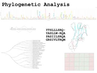
1. Steps of the phylogenetic analysis Phylogenetic analysis is an inference of evolutionary relationships between organisms. Phylogenetics tries to answer the question “How did groups of organisms come into existence?” Those relationships are usually represented by tree-like diagrams. Note: the assumption of a tree-like process of evolution is controversial!

2. Distance analyses • calculate pairwise distances • (different distance measures, correction for multiple hits, correction for codon bias) • make distance matrix (table of pairwise corrected distances) • calculate tree from distance matrix • i) using optimality criterion • (e.g.: smallest error between distance matrix • and distances in tree, or use • ii) algorithmic approaches (UPGMA or neighbor joining) B) Phylogenetic reconstruction - How

3. Parsimony analyses • find that tree that explains sequence data with minimum number of substitutions • (tree includes hypothesis of sequence at each of the nodes) • Maximum Likelihood analyses • given a model for sequence evolution, find the tree that has the highest probability under this model. • This approach can also be used to successively refine the model. • Bayesian statistics use ML analyses to calculate posterior probabilities for trees, clades and evolutionary parameters. Especially MCMC approaches have become very popular in the last year, because they allow to estimate evolutionary parameters (e.g., which site in a virus protein is under positive selection), without assuming that one actually knows the "true" phylogeny. Phylogenetic reconstruction - How

4. Elliot Sober’s Gremlins Observation: Loud noise in the attic ? Hypothesis: gremlins in the attic playing bowling Likelihood = P(noise|gremlins in the attic) P(gremlins in the attic|noise) ? ?

5. Trees – what might they mean? Calculating a tree is comparatively easy, figuring out what it might mean is much more difficult. If this is the probable organismal tree: species A species B species C species D seq. from A seq. from D seq. from C seq. from B

6. e.g., 60% bootstrap support for bipartition (AD)(CB) lack of resolution seq. from A seq. from D seq. from C seq. from B

7. the two longest branches join together e.g., 100% bootstrap support for bipartition (AD)(CB) long branch attraction artifact seq. from A seq. from D seq. from C seq. from B What could you do to investigate if this is a possible explanation? use only slow positions, use an algorithm that corrects for ASRV

8. Gene Transfer molecular tree: seq. from A seq. from D seq. from C seq. from B speciation genetransfer Gene transfer Organismal tree: species A species B species C species D

9. molecular tree: molecular tree: seq. from A seq. from A seq. from A seq. from B seq. from B seq. from C seq. from C seq. from D seq. from D seq. from D seq.’ from B seq.’ from B seq.’ from C seq.’ from C seq.’ from C gene duplication gene duplication gene duplication seq.’ from D seq.’ from D seq.’ from D Organismal tree: Gene duplication species A species B species C gene duplication species D molecular tree:

10. Gene duplication and gene transfer are equivalent explanations. The more relatives of C are found that do not have the blue type of gene, the less likely is the duplication loss scenario Ancient duplication followed by gene loss Horizontal or lateral Gene Note that scenario B involves many more individual events than A 1 HGT with orthologous replacement 1 gene duplication followed by 4 independent gene loss events

11. Function, ortho- and paralogy molecular tree: seq. from A seq.’ from B seq.’fromC seq.’ from D gene duplication seq. from B seq. from C seq. from D The presence of the duplication is a taxonomic character (shared derived character in species B C D). The phylogeny suggests that seq’ and seq have similar function, and that this function was important in the evolution of the clade BCD. seq’ in B and seq’in C and D are orthologs and probably have the same function, whereas seq and seq’ in BCD probably have different function (the difference might be in subfunctionalization of functions that seq had in A. – e.g. organ specific expression)

12. Sequence alignment: CLUSTALW MUSCLE Removing ambiguous positions: T-COFFEE FORBACK Generation of pseudosamples: SEQBOOT PROTDIST TREE-PUZZLE Calculating and evaluating phylogenies: PROTPARS PHYML NEIGHBOR FITCH SH-TEST in TREE-PUZZLE CONSENSE Comparing phylogenies: Comparing models: Maximum Likelihood Ratio Test Visualizing trees: ATV, njplot, or treeview Phylip programs can be combined in many different ways with one another and with programs that use the same file formats.

13. input and output

14. What’s in PHYLIP Programs in PHYLIP allow to do parsimony, distance matrix, and likelihood methods, including bootstrapping and consensus trees. Data types that can be handled include molecular sequences, gene frequencies, restriction sites and fragments, distance matrices, and discrete characters. Phylip works well with protein and nucleotide sequences Many other programs mimic the style of PHYLIP programs. (e.g. TREEPUZZLE, phyml, protml) Many other packages use PHYIP programs in their inner workings (e.g., PHYLO_WIN) PHYLIP runs under all operating systems Web interfaces are available

15. Programs in PHYLIP are Modular For example: SEQBOOT take one set of aligned sequences and writes out a file containing bootstrap samples. PROTDIST takes a aligned sequences (one or many sets) and calculates distance matices (one or many) FITCH (or NEIGHBOR) calculate best fitting or neighbor joining trees from one or many distance matrices CONSENSE takes many trees and returns a consensus tree …. modules are available to draw trees as well, but often people use treeview or njplot

16. is an excellent source of information. The Phylip Manual Brief one line descriptions of the programs are here The easiest way to run PHYLIP programs is via a command line menu (similar to clustalw). The program is invoked through clicking on an icon, or by typing the program name at the command line. > seqboot > protpars > fitch If there is no file called infile the program responds with: [gogarten@carrot gogarten]$ seqboot seqboot: can't find input file "infile" Please enter a new file name>

17. program folder

18. menu interface

19. Example 1 Protpars example: seqboot, protpars, consense on infile1 NOTE the bootstrap majority consensus tree does not necessarily have the same topology as the “best tree” from the original data! threshold parsimony, gap symbols - versus ? (in vi you could use :%s/-/?/g to replace all – ?) outfile outtree compare to distance matrix analysis

20. branches are scaled with respect to bootstrap support values, the number for the deepest branch is handeled incorrectly by njplot and treeview protpars (versus distance/FM) Extended majority rule consensus treeCONSENSUS TREE:the numbers on the branches indicate the numberof times the partition of the species into the two setswhich are separated by that branch occurredamong the trees, out of 100.00 trees +------Prochloroc +----------------------100.-| | +------Synechococ | | +--------------------Guillardia +-85.7-| | | | +-88.3-| +------Clostridiu | | | | +-100.-| | | | +-100.-| +------Thermoanae | +-50.8-| | | | +-------------Homo sapie +------| | | | | +------Oryza sati | | +---------------100.0-| | | +------Arabidopsi | | | | +--------------------Synechocys | | | | +---------------53.0-| +------Nostoc pun | | +-99.5-| | +-38.5-| +------Nostoc sp | | | +-------------Trichodesm | +------------------------------------------------Thermosyne remember: this is an unrooted tree!

21. ml mapping From: Olga Zhaxybayeva and J Peter Gogarten BMC Genomics 2002, 3:4 

22. ml mapping Figure 5. Likelihood-mapping analysis for two biological data sets. (Upper) The distribution patterns. (Lower) The occupancies (in percent)for the seven areas of attraction. (A) Cytochrome-b data fromref. 14. (B) Ribosomal DNA of major arthropod groups (15). From: Korbinian Strimmer and Arndt von HaeselerProc. Natl. Acad. Sci. USAVol. 94, pp. 6815-6819, June 1997

23. ml mapping (cont) If we want to know if Giardia lamblia forms the deepest branch within the known eukaryotes, we can use ML mapping to address this problem.  To apply ml mapping we choose the "higher" eukaryotes as cluster a, another deep branching eukaryote (the one that competes against Giardia) as cluster b, Giardia as cluster c, and the outgroup as cluster d.  For an example output see this sample ml-map.  An analysis of the carbamoyl phosphate synthetase domains with respect to the root of the tree of life is here.  Application of ML mapping to comparative Genome analyses see here for a comparison of different probabil;ity measures see here for an approach that solves the problem of poor taxon sampling that is usually considered inherent with quartet analyses is.

24. (a,b)-(c,d) /\ / \ / \ / 1 \ / \ / \ / \ / \ / \/ \ / 3 : 2 \ / : \ /__________________\ (a,d)-(b,c) (a,c)-(b,d)Number of quartets in region 1: 68 (= 24.3%)Number of quartets in region 2: 21 (= 7.5%)Number of quartets in region 3: 191 (= 68.2%)Occupancies of the seven areas 1, 2, 3, 4, 5, 6, 7: (a,b)-(c,d) /\ / \ / 1 \ / \ / \ / /\ \ / 6 / \ 4 \ / / 7 \ \ / \ /______\ / \ / 3 : 5 : 2 \ /__________________\ (a,d)-(b,c) (a,c)-(b,d)Number of quartets in region 1: 53 (= 18.9%) Number of quartets in region 2: 15 (= 5.4%) Number of quartets in region 3: 173 (= 61.8%) Number of quartets in region 4: 3 (= 1.1%) Number of quartets in region 5: 0 (= 0.0%) Number of quartets in region 6: 26 (= 9.3%) Number of quartets in region 7: 10 (= 3.6%) Cluster a: 14 sequencesoutgroup (prokaryotes) Cluster b: 20 sequencesother Eukaryotes Cluster c: 1 sequencesPlasmodium Cluster d: 1 sequences Giardia

25. TREE-PUZZLE – PROBLEMS/DRAWBACKS • The more species you add the lower the support for individual branches. While this is true for all algorithms, in TREE-PUZZLE this can lead to completely unresolved trees with only a few handful of sequences. • Trees calculated via quartet puzzling are usually not completely resolved, and they do not correspond to the ML-tree:The determined multi-species tree is not the tree with the highest likelihood, rather it is the tree whose topology is supported through ml-quartets, and the lengths of the resolved branches is determined through maximum likelihood.

26. ml mapping (cont) If we want to know if Giardia lamblia forms the deepest branch within the known eukaryotes, we can use ML mapping to address this problem.  To apply ml mapping we choose the "higher" eukaryotes as cluster a, another deep branching eukaryote (the one that competes against Giardia) as cluster b, Giardia as cluster c, and the outgroup as cluster d.  For an example output see this sample ml-map.  An analysis of the carbamoyl phosphate synthetase domains with respect to the root of the tree of life is here.  Application of ML mapping to comparative Genome analyses see here for a comparison of different probabil;ity measures see here for an approach that solves the problem of poor taxon sampling that is usually considered inherent with quartet analyses is.

27. Li pi= L1+L2+L3 Ni pi Ntotal Alternative Approaches to Estimate Posterior Probabilities Bayesian Posterior Probability Mapping with MrBayes(Huelsenbeck and Ronquist, 2001) Problem: Strimmer’s formula only considers 3 trees (those that maximize the likelihood for the three topologies) Solution: Exploration of the tree space by sampling trees using a biased random walk (Implemented in MrBayes program) Trees with higher likelihoods will be sampled more often ,where Ni - number of sampled trees of topology i, i=1,2,3 Ntotal – total number of sampled trees (has to be large)

28. Illustration of a biased random walk Figure generated using MCRobot program (Paul Lewis, 2001)

29. selection versus drift see Kent Holsinger’s java simulations at http://darwin.eeb.uconn.edu/simulations/simulations.html The law of the gutter. compare drift versus select + drift The larger the population the longer it takes for an allele to become fixed. Note: Even though an allele conveys a strong selective advantage of 10%, the allele has a rather large chance to go extinct. Note#2: Fixation is faster under selection than under drift. BUT

30. s=0 Probability of fixation, P, is equal to frequency of allele in population. Mutation rate (per gene/per unit of time) = u ;   freq. with which allele is generated in diploid population size N =u*2N Probability of fixation for each allele = 1/(2N) Substitution rate = frequency with which new alleles are generated * Probability of fixation= u*2N *1/(2N) = u Therefore: If f s=0, the substitution rate is independent of population size, and equal to the mutation rate !!!! (NOTE: Mutation unequal Substitution! )This is the reason that there is hope that the molecular clock might sometimes work. Fixation time due to drift alone: tav=4*Ne generations  (Ne=effective population size; For n discrete generations Ne= n/(1/N1+1/N2+…..1/Nn)

31. s>0 Time till fixation on average: tav= (2/s) ln (2N) generations (also true for mutations with negative “s” ! discuss among yourselves) E.g.:  N=106, s=0:  average time to fixation: 4*106 generationss=0.01:  average time to fixation: 2900 generations  N=104, s=0:  average time to fixation: 40.000 generationss=0.01:  average time to fixation: 1.900 generations  => substitution rate of mutation under positive selection is larger than the rate wite which neutral mutations are fixed.

32. Random Genetic Drift Selection 100 advantageous Allele frequency disadvantageous 0 Modified from from www.tcd.ie/Genetics/staff/Aoife/GE3026/GE3026_1+2.ppt

33. Positive selection • A new allele (mutant) confers some increase in the fitness of the organism • Selection acts to favour this allele • Also called adaptive selection or Darwinian selection. NOTE: Fitness = ability to survive and reproduce Modified from from www.tcd.ie/Genetics/staff/Aoife/GE3026/GE3026_1+2.ppt

34. Advantageous allele Herbicide resistance gene in nightshade plant Modified from from www.tcd.ie/Genetics/staff/Aoife/GE3026/GE3026_1+2.ppt

35. Negative selection • A new allele (mutant) confers some decrease in the fitness of the organism • Selection acts to remove this allele • Also called purifying selection Modified from from www.tcd.ie/Genetics/staff/Aoife/GE3026/GE3026_1+2.ppt

36. Deleterious allele Human breast cancer gene, BRCA2 5% of breast cancer cases are familial Mutations in BRCA2 account for 20% of familial cases Normal (wild type) allele Mutant allele (Montreal 440 Family) Stop codon 4 base pair deletion Causes frameshift Modified from from www.tcd.ie/Genetics/staff/Aoife/GE3026/GE3026_1+2.ppt

37. Neutral mutations • Neither advantageous nor disadvantageous • Invisible to selection (no selection) • Frequency subject to ‘drift’ in the population • Random drift – random changes in small populations

38. Types of Mutation-Substitution • Replacement of one nucleotide by another • Synonymous (Doesn’t change amino acid) • Rate sometimes indicated by Ks • Rate sometimes indicated by ds • Non-Synonymous (Changes Amino Acid) • Rate sometimes indicated by Ka • Rate sometimes indicated by dn (this and the following 4 slides are from mentor.lscf.ucsb.edu/course/ spring/eemb102/lecture/Lecture7.ppt)

39. Genetic Code – Note degeneracy of 1st vs 2nd vs 3rd position sites

40. Genetic Code Four-fold degenerate site – Any substitution is synonymous From: mentor.lscf.ucsb.edu/course/spring/eemb102/lecture/Lecture7.ppt

41. Genetic Code Two-fold degenerate site – Some substitutions synonymous, some non-synonymous From: mentor.lscf.ucsb.edu/course/spring/eemb102/lecture/Lecture7.ppt

42. Measuring Selection on Genes • Null hypothesis = neutral evolution • Under neutral evolution, synonymous changes should accumulate at a rate equal to mutation rate • Under neutral evolution, amino acid substitutions should also accumulate at a rate equal to the mutation rate From: mentor.lscf.ucsb.edu/course/spring/eemb102/lecture/Lecture7.ppt

43. Counting #s/#a Ser Ser Ser Ser Ser Species1 TGA TGC TGT TGT TGT Ser Ser Ser Ser Ala Species2 TGT TGT TGT TGT GGT #s = 2 sites #a = 1 site #a/#s=0.5 To assess selection pressures one needs to calculate the rates (Ka, Ks), i.e. the occurring substitutions as a fraction of the possible syn. and nonsyn. substitutions. Things get more complicated, if one wants to take transition transversion ratios and codon bias into account. See chapter 4 in Nei and Kumar, Molecular Evolution and Phylogenetics. Modified from: mentor.lscf.ucsb.edu/course/spring/eemb102/lecture/Lecture7.ppt

44. dambe Two programs worked well for me to align nucleotide sequences based on the amino acid alignment, One is DAMBE (only for windows). This is a handy program for a lot of things, including reading a lot of different formats, calculating phylogenies, it even runs codeml (from PAML) for you. The procedure is not straight forward, but is well described on the help pages. After installing DAMBE go to HELP -> general HELP -> sequences -> align nucleotide sequences based on …-> If you follow the instructions to the letter, it works fine. DAMBE also calculates Ka and Ks distances from codon based aligned sequences.

45. aa based nucleotide alignments (cont) An alternative is the tranalign program that is part of the emboss package. On bbcxsrv1 you can invoke the program by typing tranalign. Instructions and program description are here . If you want to use your own dataset in the lab on Monday, generate a codon based alignment with either dambe or tranalign and save it as a nexus file and as a phylip formated multiple sequence file (using either clustalw, PAUP (export or tonexus), dambe, or readseq on the web)

46. PAML (codeml) the basic model

47. sites versus branches You can determine omega for the whole dataset; however, usually not all sites in a sequence are under selection all the time. PAML (and other programs) allow to either determine omega for each site over the whole tree, , or determine omega for each branch for the whole sequence, . It would be great to do both, i.e., conclude codon 176 in the vacuolar ATPases was under positive selection during the evolution of modern humans – alas, a single site does not provide any statistics ….

48. Sites model(s) work great have been shown to work great in few instances. The most celebrated case is the influenza virus HA gene. A talk by Walter Fitch (slides and sound) on the evolution ofthis molecule is here . This article by Yang et al, 2000 gives more background on ml aproaches to measure omega. The dataset used by Yang et al is here: flu_data.paup .

49. MrBayes analyzing the *.nex.p file • The easiest is to load the file into excel (if your alignment is too long, you need to load the data into separate spreadsheets – see here execise 2 item 2 for more info) • plot LogL to determine which samples to ignore • for each codon calculate the the average probability (from the samples you do not ignore) that the codon belongs to the group of codons with omega>1. • plot this quantity using a bar graph.

50. the same after rescaling the y-axis plot LogL to determine which samples to ignore