Download
1 / 35
350 likes | 597 Views
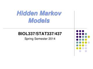
Hidden Markov Models Supplement to the Probabilistic Graphical Models Course 2009 School of Computer Science and Engineering Seoul National University. Summary of Chapter 7: P. Baldi and S. Brunak, Bioinformatics: The Machine Learning Approach, MIT Press, 1998. Outline. Introduction

E N D
Hidden Markov ModelsSupplement to the Probabilistic Graphical Models Course 2009School of Computer Science and EngineeringSeoul National University Summary of Chapter 7: P. Baldi and S. Brunak, Bioinformatics: The Machine Learning Approach, MIT Press, 1998
Outline • Introduction • Prior Information and Initialization • Likelihood and Basic Algorithms • Learning Algorithms • Application of HMMs: General Aspects (C) 2001 SNU Biointelligence Lab
Hidden Markov Model (HMM): Definition • First order discrete HMM: stochastic generative model for time series • S: set of states • A: discrete alphabet of symbols • T = (tji): transition probability matrix, tji = P(St+1= j | St = i) • E = (eix): emission probability matrix, eix= P(X | St = i) • First order assumption: The emission and transition depend on the current state only, not on the entire previous states. • Meaning of “Hidden” • Only emitted symbols are observable. • Random walk between states are hidden. (C) 2001 SNU Biointelligence Lab
0.5 0.25 0.25 0.25 0.25 0.5 S 0.25 0.25 E 0.5 0.1 0.1 0.1 0.7 0.5 ATCCTTTTTTTCA HMM: Example 0.25 0.25 (C) 2001 SNU Biointelligence Lab
HMMs for Biological Sequences (1) • Example of symbols in biological sequence application • 20-letter amino acid alphabet for protein sequences • 4-letter nucleotide alphabet for DNA/RNA sequences • Standard HMM architecture S = {start, m1, …, mN, i1,…,iN+1, d1,…, dN, end} • start, end • main states • insert states • delete states • N: length of model, typically average length of the sequences in the family (C) 2001 SNU Biointelligence Lab
HMMs for Biological Sequences (2) di S mi E ii Figure 7.2 : The Standard HMM Architecture. S is the start state, E is the end state, and di, mi and ii denote delete, main, and insert state, respectively. (C) 2001 SNU Biointelligence Lab
Three Questions in HMM • Likelihood question • How likely is this sequence for this HMM? • Decoding question • What is the most probable sequence of transitions and emissions through the HMM underlying the production of this particular sequence? • Learning question • How should their values be revised in light of the observed sequence? Given a sequence O1, O2, …, Or find Given a sequence O1, O2, …, Or find Given sequences {O1, O2, …, On} find (C) 2001 SNU Biointelligence Lab
Prior Information and Initialization • Once the architecture is selected, one can further restrain the freedom of the parameters if the corresponding information is available. • In the Bayesian approach, this background information can be incorporated by priors. • Because of the multinomial models associated with HMM emissions and transitions, the natural priors on HMM parameters are Dirichlet distributions (Chap. 2). • Dirichlet priors on transitions: • Dirichlet priors on emissions: (C) 2001 SNU Biointelligence Lab
Initialization of Parameters • Different methods • Unform • Random • Average composition • Uniform initialization without a prior that favors transitions toward the main states is not, in general, a good idea. • Figure 7.3: Main states have a lower fan-out (3) than insert or delete states (4). • Multiple alignment can be used to initialize the parameters prior to learning. • E.g.: assigning a main state to any column of the alignment that contains less than 50% gaps. (C) 2001 SNU Biointelligence Lab
Likelihood and Basic Algorithm • Likelihood of a sequence O according to HMM M=M(w) • O = X1…Xt…XT : sequence of emission • M(w) : HMM with parameter w • Path in M: sequence of consecutive states in which emitting states emit the corresponding letter. (7.1) • Likelihood equation • Difficulty of direct manipulation of likelihood equation • Number of paths is typically exponential! • Forward-algorithm: avoiding looking at all possible hidden paths (C) 2001 SNU Biointelligence Lab
Forward-Backward Algorithm: Basic Concept • Forward pass: • Define • Probability of subsequence O1, O2, …, Ot when in Siat t Note: any path must be in one of N states at t 1 2 … … … … … … … N t-1 t T 1 (C) 2001 SNU Biointelligence Lab
Forward-Backward Algorithm • Notice • Define an analogues backward pass so that: and … … … … … t-1 t t+1 Forward:j i Backward:i j (C) 2001 SNU Biointelligence Lab
The Forward Algorithm (1) • Objective: • Algorithm: • The probability of being in state i at time t, having observed the letters X1…Xt in the model M(w) • For delete states, • Convergence in the case of delete states (Appendix D) (C) 2001 SNU Biointelligence Lab
The Forward Algorithm (2) • Silent path from j to i • If the only internal nodes in the path are delete (silent) states. • tijD : the probability of moving from j to i silently. • Forward variables for delete states • E : all emitting states • Relationship with other algorithms • Forward propagation as in a linear neural network: with T layers (each time step) and N units in each layer (one for each HMM states) • An HMM can be viewed as a dynamic mixture model • Probability of emitting the letter Xt : (C) 2001 SNU Biointelligence Lab
The Backward Algorithm (1) • Objective: the reverse of the forward algorithm • Backward variable: the probability of being in state i at time t, with partial observation of the sequence from Xt+1 to end. • Propagation equation for emitting states • Propagation equation for delete states (C) 2001 SNU Biointelligence Lab
The Backward Algorithm (2) • Using the forward and backward variables, we can compute the probability i(t) of being in state i at time t, given the observation sequence Oand the model w. • Probability ji(t)of using i j transition at time t. • Also (C) 2001 SNU Biointelligence Lab
The Viterbi Algorithm • Objective: Find the most probable path accounting for the first t symbols of O and terminating in state i. • i(t) : a prefix path, with emissions X1,…,Xt ending in state i. • Propagation • For emitting states • For deleting states (C) 2001 SNU Biointelligence Lab
Computing Expectations • Posterior distribution Q() = P( |O,w) • For learning, some expectations needs to be calculated. • n(i, , O): the number of times i is visited, given and O • n(i, X, , O): the number of times the letter X is emitted from i, given and O • n(j, i, X, , O): the number of times the i j transition is used, given and O (C) 2001 SNU Biointelligence Lab
Learning Algorithms (1) • HMM training algorithms • Baum-Welch or EM algorithm • Gradient-descent algorithms • Generalized EM algorithms • Simulated annealing • Markov chain Monte Carlo • … • We concentrate on the first level of Bayesian inference, i.e. MAP estimation, proceeding as follows: • ML with on-line learning (given one sequence) • ML with batch learning (with multiple sequences) • MAP (considering priors) \ (C) 2001 SNU Biointelligence Lab
Learning Algorithms (2) • Consider the likelihood: • Lagrangian optimization function of ML (7.22) • i, i : Lagrange multipliers from normalization constraints • From (7.1) , we have (7.23) • By setting the partial derivative of L to 0, at the optimum we must have (C) 2001 SNU Biointelligence Lab
Learning Algorithms (3) • By summing over all alphabet letters, • At the optimum, we must have (in case of emission probability) (7.26) • ML equation cannot be solved directly since the posterior distribution Q depends on the values of eiX • EM algorithms can do it. • First, estimate Q() = P( |O,w) • Second, update parameters using (7.26) (C) 2001 SNU Biointelligence Lab
EM Algorithm (1): Baum-Welch • We define the energy over hidden configurations (Chs. 3 and 4) as • EM is then defined as an iterative double minimization process of the function (i.e., free energy at temperature 1) w.r.t. Q and w • First step, calculate Q • Second step, minimize F, with respect to w, with Q()fixed. Since the entropy term H is independent of w, we minimize the Lagrangean: (C) 2001 SNU Biointelligence Lab
EM Algorithm (2): Baum-Welch • Following similar steps as before (Eqns. 7.23-7.25), we obtain the EM reestimation equations • In words, the statistic is the expected number of times in state i observing symbol X, divided by the expected number of times in state i. • Forward-backward procedures can calculate above statistics. (emmission) (transition) (C) 2001 SNU Biointelligence Lab
Batch EM Algorithm • In the case of K sequences O1,…,OK • Online use of EM can be problematic. • No learning rate available and the EM can take large steps in the descent direction, leading to poor local minima. • ‘Carpet jumping’ effect (C) 2001 SNU Biointelligence Lab
Gradient Descent (1) • Reparameterize HMM using normalized exponentials, with new variables wiX, wij. • Advantage 1: Automatically preserving normalization constrains • Advantage 2: Never reaching zero probabilities. • Partial derivatives (C) 2001 SNU Biointelligence Lab
Gradient Descent (2) • Chain rule: • On-line gradient descent: • Remarks • For MAP estimation, add the derivative of the log prior. • O(KN2) operations per training cycle. • Just like EM, one forward and backward propagation are needed per iteration. • Unlike EM, online gradient-descent is a smooth algorithm: unlearning (reversing the effect of gradient descent) is easy. (C) 2001 SNU Biointelligence Lab
Viterbi Learning (1) • Idea: Focus on the most likely one path with each sequence • EM and gradient descent update equation: expectation over all possible hidden paths. • Replace: n(i, X, , O) n(i, X, *(O)) • In standard architecture, n(i, X, *(O)) = 0 or 1, except for insert states. • On-line Viterbi EM makes little sense: mostly updated to 0 or 1 • On-line gradient descent, at each step along a Viterbi path, and for any state i on the path, update the parameters. • Eix = 1 (Tji = 1) if emission of X from i (i j transition) is used. (C) 2001 SNU Biointelligence Lab
Viterbi Learning (2) • Remark 1 • Quick approximation to the corresponding non-Viterbi version. • Speed up of order of factor 2: *(O) with no backward propagation • Remark 2 • Crude approximation • Likelihoods in general are not sharply peaked around a single optimal path • Remark 3 • Minimizing a different objective function (C) 2001 SNU Biointelligence Lab
Other Aspects (1) • Scaling • Machine precision vs. P(|O,w) • Some techniques to avoid underflow are needed. • Learning the Architecture • [389]: merge states from complex model. • [142]: small starting point; deleting transitions with low probability; duplicating most connected states. • Good results in small test cases, but unlikely in practice • Adaptable Model Length • Adaptation of N of average length of the sequences being modeled. • [251]: “surgery” algorithm • 50% used insert state: replace it with new main state (together with corresponding new delete and insert state.) • 50% used delete state: remove it together with corresponding main and insert states. (C) 2001 SNU Biointelligence Lab
Other Aspects (2) • Architectural Variations • The variations of standard architecture. • Multiple HMM architecture, loop and wheel are introduced in Chapter 8. • Ambiguous Symbols • The reason of adoption of ambiguous symbols: imperfect sequencing techniques. (C) 2001 SNU Biointelligence Lab
Applications of HMMs: General Aspects • Successfully derived from a family of sequences. • For any given sequence • The computation of its probability according to the model as well as its most likely associated path • Aanalysis of the model structure. • Applications • Multiple alignments • Database mining and classification of sequence and fragments • Structural analysis and pattern discovery (C) 2001 SNU Biointelligence Lab
Multiple Alignments (1) • Aligning the Viterbi paths to each other. • Computing the Viterbi path of a sequence: “aligning a sequence to the model” • O(KN2): when multiple alignment of K sequences. • O(NK): in case of multi-dimensional dynamic programming • Rich expression power against conventional methods • Gap: deletion in the second sequence of insertion in the first sequence Two distinct sets of Viterbi paths in HMM • Conventional methods can not distinguish. • HMM becomes conventional techniques if N is fixed to length of longest sequence and all insert states are removed. (C) 2001 SNU Biointelligence Lab
Multiple Alignments (2) • Insert and delete states of HMM represent formal operations on sequences. • Whether and how they can be related to evolutionary events? • Phylogenetic trees?: require tree structure as well as a clear notion of substitution (Chapter 10) • Full Bayesian treatment is nearly intractable in HMM. (C) 2001 SNU Biointelligence Lab
Database Mining and Classification • The likelihood score of any given sequence can be used for the purpose of discriminative test and database search. • For classification • Training a model for each class. • Give class label to the largest likelihood score. (C) 2001 SNU Biointelligence Lab
Structural Analysis and Pattern Discovery • Information or new pattern is discovered by examining the structure of a trained HMM. • High emission or transition probabilities are usually associated with conserved regions or consensus patterns. • One technique: plot the entropy of the emission distributions along the backbone of the model. • Initial weak detection can guide the design of more specialized architectures (Chapter 8). (C) 2001 SNU Biointelligence Lab