One-Way ANOVA
One-Way ANOVA. Introduction to Analysis of Variance (ANOVA). What is ANOVA?. ANOVA is short for ANalysis Of VAriance Used with 3 or more groups to test for MEAN DIFFS. E.g., caffeine study with 3 groups: No caffeine Mild dose Jolt group Level is value, kind or amount of IV


One-Way ANOVA
E N D
Presentation Transcript
One-Way ANOVA Introduction to Analysis of Variance (ANOVA)
What is ANOVA? • ANOVA is short for ANalysis Of VAriance • Used with 3 or more groups to test for MEAN DIFFS. • E.g., caffeine study with 3 groups: • No caffeine • Mild dose • Jolt group • Level is value, kind or amount of IV • Treatment Group is people who get specific treatment or level of IV • Treatment Effect is size of difference in means
Rationale for ANOVA (1) • We have at least 3 means to test, e.g., H0: 1 = 2 = 3. • Could take them 2 at a time, but really want to test all 3 (or more) at once. • Instead of using a mean difference, we can use the variance of the group means about the grand mean over all groups. • Logic is just the same as for the t-test. Compare the observed variance among means (observed difference in means in the t-test) to what we would expect to get by chance.
Rationale for ANOVA (2) Suppose we drew 3 samples from the same population. Our results might look like this: Note that the means from the 3 groups are not exactly the same, but they are close, so the variance among means will be small.
Rationale for ANOVA (3) Suppose we sample people from 3 different populations. Our results might look like this: Note that the sample means are far away from one another, so the variance among means will be large.
Rationale for ANOVA (4) Suppose we complete a study and find the following results (either graph). How would we know or decide whether there is a real effect or not? To decide, we can compare our observed variance in means to what we would expect to get on the basis of chance given no true difference in means.
Review • When would we use a t-test versus 1-way ANOVA? • In ANOVA, what happens to the variance in means (between cells) if the treatment effect is large?
Rationale for ANOVA We can break the total variance in a study into meaningful pieces that correspond to treatment effects and error. That’s why we call this Analysis of Variance. Definitions of Terms Used in ANOVA: The Grand Mean, taken over all observations. The mean of any level of a treatment. The mean of a specific level (1 in this case) of a treatment. The observation or raw data for the ith person.
The ANOVA Model A treatment effect is the difference between the overall, grand mean, and the mean of a cell (treatment level). Error is the difference between a score and a cell (treatment level) mean. The ANOVA Model: An individual’s score A treatment or IV effect The grand mean is + Error +
The ANOVA Model The grand mean A treatment or IV effect Error The graph shows the terms in the equation. There are three cells or levels in this study. The IV effect and error for the highest scoring cell is shown.
ANOVA Calculations Sums of squares (squared deviations from the mean) tell the story of variance. The simple ANOVA designs have 3 sums of squares. The total sum of squares comes from the distance of all the scores from the grand mean. This is the total; it’s all you have. The within-group or within-cell sum of squares comes from the distance of the observations to the cell means. This indicates error. The between-cells or between-groups sum of squares tells of the distance of the cell means from the grand mean. This indicates IV effects.
In the total sum of squares, we are finding the squared distance from the Grand Mean. If we took the average, we would have a variance.
Within sum of squares refers to the variance within cells. That is, the difference between scores and their cell means. SSW estimates error.
The between sum of squares relates the Cell Means to the Grand Mean. This is related to the variance of the means.
ANOVA Source Table (2) • df – Degrees of freedom. Divide the sum of squares by degrees of freedom to get • MS, Mean Squares, which are population variance estimates. • F is the ratio of two mean squares. F is another distribution like z and t. There are tables of F used for significance testing.
Review • What are critical values of a statistics (e.g., critical values of F)? • What are degrees of freedom? • What are mean squares? • What does MSW tell us?
Set alpha (.05). State Null & Alternative H0: H1: not all are =. Calculate test statistic: F=12.5 Determine critical value F.05(2,12) = 3.89 Decision rule: If test statistic > critical value, reject H0. Decision: Test is significant (12.5>3.89). Means in population are different. Review 6 Steps
Post Hoc Tests • If the t-test is significant, you have a difference in population means. • If the F-test is significant, you have a difference in population means. But you don’t know where. • With 3 means, could be A=B>C or A>B>C or A>B=C. • We need a test to tell which means are different. Lots available, we will use 1.
Tukey HSD (1) Use with equal sample size per cell. HSD means honestly significant difference. is the Type I error rate (.05). Is a value from a table of the studentized range statistic based on alpha, dfW (12 in our example) and k, the number of groups (3 in our example). Is the mean square within groups (10). Is the number of people in each group (5). MSW Result for our example. From table
Tukey HSD (2) To see which means are significantly different, we compare the observed differences among our means to the critical value of the Tukey test. The differences are: 1-2 is 79-84 = -5 (say 5 to be positive). 1-3 is 79-74 = 5 2-3 is 84-74 = 10. Because 10 is larger than 5.33, this result is significant (2 is different than 3). The other differences are not significant. Review 6 steps.
Review • What is a post hoc test? What is its use? • Describe the HSD test. What does HSD stand for?
Test • Another name for mean square is _________. • standard deviation • sum of squares • treatment level • variance
Test When do we use post hoc tests? • a. after a significant overall F test • b. after a nonsignificant overall F test • c. in place of an overall F test • d. when we want to determine the impact of different factors