Download

1 / 22
280 likes | 580 Views
DFT – Practice Simple Molecules & Solids [based on Chapters 5 & 2, Sholl & Steckel]. Input files Supercells Molecules Solids. The DFT prescription for the total energy (including geometry optimization). Guess ψ ik (r) for all the electrons. Self-consistent field (SCF) loop. Solve!. No.

E N D
DFT – PracticeSimple Molecules & Solids[based on Chapters 5 & 2, Sholl & Steckel] • Input files • Supercells • Molecules • Solids
The DFT prescription for the total energy(including geometry optimization) Guess ψik(r) for all the electrons Self-consistent field (SCF) loop Solve! No Is new n(r) close to old n(r) ? Yes Geometry optimization loop Calculate total energy E(a1,a2,a3,R1,R2,…RM) = Eelec(n(r); {a1,a2,a3,R1,R2,…RM}) + Enucl Calculate forces on each atom, and stress in unit cell Move atoms; change unit cell shape/size No Are forces and stresses zero? Yes DONE!!!
Approximations Approximation 1: finite number of k-points Approximation 2: representation of wave functions Approximation 3: pseudopotentials Approximation 4: exchange-correlation
Required input in typical DFT calculations VASP input files • Initial guesses for the unit cell vectors (a1, a2, a3) and positions of all atoms (R1, R2, …, RM) • k-point mesh to “sample” the Brillouin zone • Pseudopotential for each atom type • Basis function information (e.g., plane wave cut-off energy, Ecut) • Level of theory (e.g., LDA, GGA, etc.) • Other details (e.g., type of optimization and algorithms, precision, whether spins have to be explicitly treated, etc.) POSCAR KPOINTS POTCAR INCAR
The general “supercell” • Initial geometry specified by the periodically repeating unit “Supercell”, specified by 3 vectors {a1, a2, a3} • Each supercell vector specified by 3 numbers • Atoms within the supercell specified by coordinates {R1, R2, …, RM} • Supercells allow for a unified treatment of isolated atoms & molecules, defect-free & defective solids (i.e., point defects, surfaces/interfaces, and 0-d, 1-d, 2-d & 3-d systems); How? a3 = a3xi + a3yj + a3zk a1 = a1xi + a1yj + a1zk a2 = a2xi + a2yj + a2zk
More on supercells (in 2-d) Primitive cell Wigner-Seitz cell
The simple cubic “supercell” • Applicable to real simple cubic systems, and molecules • May be specified in terms of the lattice parameter a a3 = ak a1 = ai a2 = aj
The FCC “supercell” • The primitive lattice vectors are not orthogonal • In the case of simple metallic systems, e.g., Cu only one atom per primitive unit cell • Again, in terms of the lattice parameter a a3 = 0.5(i + k) a2 = 0.5a(j + k) a1 = 0.5a(i + j)
Diatomic molecule, A-B Only one degree of freedom RAB If we new E(RAB), then we can determine potential energy surface (PES) Energy RAB Curvature = mw2 m = mAmB/(mA+mB) Note: slope = -force Bond energy R0 Thus, IF E(RAB) is known, then we can trivially determine equilibrium bond length, bond energy and vibrational frequency!
Isolated diatomic molecules • Lets consider a homonuclear diatomic molecule • a >> d (i.e., a ~ 10 A) • We need to compute energy versus bond length • Note: vibrational frequency computations requires accuracy … as frequency is related to curvature in the “harmonic” part of the E vs. d curve [Chapter 5] • What about k-point sampling? a3 = ak d a1 = ai a2 = aj
Example – Cl2 • Energy versus bond length of Cl2 Curvature needs to be evaluated accurately to yield frequency [Chapter 5, Table 5.1] Experiment
Bulk cubic material Only one degree of freedom lattice parameter a, or Volume V (= a3) If we new E(V), then we can determine potential energy surface (PES) Energy V Curvature = B/V0 B = bulk modulus Note: slope = stress Cohesive energy V0 Thus, IF E(V) is known [equation of state], then we can trivially determine equilibrium lattice parameter, cohesive energy and bulk modulus!
FCC solids • We will consider primitive cells of simple FCC systems (Cu) • We will determine the equilibrium lattice parameter of Cu and bulk modulus • What about k-point sampling? • The proper number of k-points in each direction needs to be determined convergence
Example – FCC Cuk-point sampling • Remember: Integration over the Brillouin zone (BZ) replaced by a summation • The Monkhorst-Pack scheme requires specification of 3 integers, representing the number of k-points along each of the 3 axis Converged!
Equation of State (EOS)The Harmonic Solid • A harmonic or “Hooke” solid is characterized by the “equation of state” (Note: For an ideal gas: PV = NRT) • Combined with the thermodynamic relations … • … we get the equilibrium bulk modulus, B0 = V0*d2E/dV2|V0 • In other words, fitting the DFT energy vs volume results to the above EOS will yield E0, V0 and B0 (as long as we are close to the minimum harmonic limit)
A better 2nd order EOS(“pseudoharmonic” approximation) • Note that the bulk modulus is not a constant at all volumes or pressures for a harmonic solid, as B = V*d2E/dV2|V0 • If we require that the bulk modulus remains a constant at all pressures or volumes, we have
The Murnaghan 3rd order EOS • If we allow for the (known) fact that the bulk modulus does depend on pressure, but that the first pressure derivative is a constant • By fitting the DFT E vs. V data to the above equation, we can determine E0, V0, B0 and B0’
Comparison of various EOS forms • Relative energy per volume vs. scaled volume, for B0 = 1, B0’ = 3.5 • For accurate determination of B0 and B0’, one will need to use Murnaghan EOS • Fitting DFT energy vs. volume will yield B0 and B0’ • For most practical purposes, using the harmonic fit will be sufficient (as long as we are sufficiently close to the minimum), as we will do …
Example – FCC CuEnergy versus lattice parameter • Perform quadratic fit: xa2 + ya + z • Minimum in energy at a0 = –y/(2x) = 3.64 Å (expt: 3.61 Å) • Bulk modulus, B = -(16/9)*(x2/y) = 146 GPa (expt: 140 GPa) • Why? B = V0*d2E/dV2|V0 = (4/9a0)*d2E/da2|a0 = -(16/9)*(x2/y) Experiment
Bulk Silicon [Yin and Cohen, PRB 26, 5668 (1982)] Slope is transformation pressure Why? G = E + PV –TS DG = DE + PDV (DS = 0) Transformation at DG = 0 P = -DE/DV
Expt value Expt value Expt value Bulk Iron • DFT-LDA gives the wrong description of bulk iron it predicts that the non-magnetic FCC structure is the most stable state! • One has to use DFT-GGA to get things right • DFT-GGA also does better with magnetic moment • Note: spin-polarized calculations help address magnetic phenomena • Note: FM ferro-magnetic; PM para-magnetic (or non-magnetic)
Anomaly in metallic crystal structure – Polonium(vis a vis the Kepler conjecture!)


![DFT Practice Simple Molecules Solids [based on Chapters 5 2, Sholl Steckel]](https://cdn4.slideserve.com/776083/slide1-dt.jpg)


![Thermal Behavior – II Free Energy & Phase Diagrams [partly based on Chapter 7, Sholl & Steckel]](https://cdn1.slideserve.com/3337775/thermal-behavior-ii-free-energy-phase-diagrams-partly-based-on-chapter-7-sholl-steckel-dt.jpg)

![DFT – Practice Surface Science [based on Chapter 4, Sholl & Steckel]](https://cdn2.slideserve.com/3753679/dft-practice-surface-science-based-on-chapter-4-sholl-steckel-dt.jpg)