Understanding Short-Run and Long-Run Cost Relationships in Microeconomics
This microeconomics exercise demonstrates the relationship between short-run and long-run costs using the Lagrangean method for cost minimization. The long-run cost analysis shows constant returns to scale with a homogeneous production function, leading to constant average costs. The short-run analysis incorporates fixed factors and establishes the short-run cost function through first-order conditions (FOCs). The approach includes graphing isoquants and deriving supply curves by manipulating the relationship between price and marginal cost, emphasizing the utility of constant returns to scale (CRTS) in simplifying computations.

Understanding Short-Run and Long-Run Cost Relationships in Microeconomics
E N D
Presentation Transcript
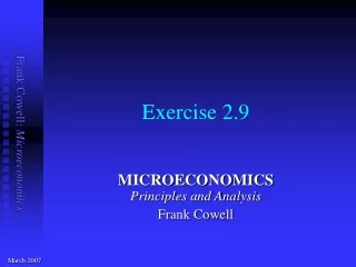
Exercise 2.9 MICROECONOMICS Principles and Analysis Frank Cowell March 2007
Ex 2.9(1): Question • purpose: demonstrate relationship between short and long run • method: Lagrangean approach to cost minimisation. First part can be solved by a “trick”
Ex 2.9(1): Long-run costs • Production function is homogeneous of degree 1 • increase all inputs by a factor t > 0 (i.e. z→tz)… • …and output increases by the same factor (i.e. q→tq) • constant returns to scale in the long run • CRTS implies constant average cost • C(w, q) / q = A (a constant) • so C(w, q) = Aq • differentiating: Cq(w, q) = A • So LRMC = LRAC = constant • Their graphs will be an identical straight line
Ex 2.9(2): Question method: • Standard Lagrangean approach
Ex 2.9(2): short-run Lagrangean • In the short run amount of good 3 is fixed • z3 = `z3 • Could write the Lagrangean as • But it is more convenient to transform the problem thus • where
z2 z1 Ex 2.9(2): Isoquants • Sketch the isoquant map • Isoquants do not touch the axes • So maximum problem must have an interior solution
Ex 2.9(2): short-run FOCs • Differentiating Lagrangean, the FOCS are • This implies • To find conditional demand function must solve for l • use the above equations… • …and the production function
Ex 2.9(2): short-run FOCs (more) • Using FOCs and the production function: • This implies • where • This will give us the short-run cost function
Ex 2.9(2): short-run costs • By definition, short-run costs are: • This becomes • Substituting for k: • From this we get • SRAC: • SRMC:
q Ex 2.9(2): short-run MC and AC marginal cost average cost
Ex 2.9(3): Question method: • Draw the standard supply-curve diagram • Manipulate the relationship p = MC
p q Ex 2.9(3): short-run supply curve • average cost curve • marginal cost curve • minimum average cost • supply curve p q
Ex 2.9(3): short-run supply elasticity • Use the expression for marginal cost: • Set p = MC for p≥p • Rearrange to get supply curve • Differentiate last line to get supply elasticity
Ex 2.9: Points to remember • Exploit CRTS to give you easy results • Try transforming the Lagrangean to make it easier to manipulate • Use MC curve to derive supply curve