Hypotheses about Contrasts
250 likes | 512 Views
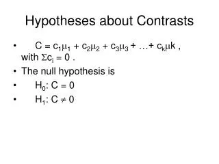
Hypotheses about Contrasts. C = c 1 1 + c 2 2 + c 3 3 + …+ c k k , with c i = 0 . The null hypothesis is H 0 : C = 0 H 1 : C 0. Hypotheses about Contrasts. C 1 = (0) instruction + (1) advance organizer (-1) neutral topic

Hypotheses about Contrasts
E N D
Presentation Transcript
Hypotheses about Contrasts • C = c11 + c22 + c33 + …+ ckk , with ci = 0 . • The null hypothesis is • H0: C = 0 • H1: C 0
Hypotheses about Contrasts • C1 = (0)instruction + (1)advance organizer (-1)neutral topic • Thus, for this contrast we ignore the straight instruction condition, as evidenced by its weight of 0, and subtract the mean of the neutral topic condition from the mean for the advance organizer condition. A second contrast might be 2, -1, -1: • C2 = (2)instruction (-1)advance organizer (-1)neutral topic • We can interpret this contrast better by examining its null hypothesis: • C2 = 0 • = (2)instruction (-1)advance organizer (-1)neutral topic , • so that • (2)instruction = (1)advance organizer + (1)neutral topic • and • instruction - [ (1)advance organizer – (1)neutral topic ] / 2 = 0 .
Contrasts • simple contrasts, if only two groups have nonzero coefficients, and • complex contrasts for those involving three or more groups
Planned Orthogonal Contrasts • Orthogonal contrasts have the property that they are mathematically independent of each other. That is, there is no information in one that tells us anything about the other. This is created mathematically by requiring that for each pair of contrasts in the set, • ci1ci2 = 0, • where ci1 is the contrast value for group i in contrast 1, ci2 the contrast value for the same group in contrast 2. For example, with C1 and C2 above, • C1 : 0 1 -1 • C2: 2 -1 -1 • C1C2: 0 x 2 + 1 x –1 + -1 x –1 = 0 –1 + 1 • = 0
Planned Orthogonal Contrasts • VENN DIAGRAM REPRESENTATION SSc2 Treat SS SSy R2c1=SSc1/SSy R2c2=SSc2/SSy R2y=(SSc1+SSc2)/SSy SSerror SSc1
Geometry of POCs GP 2 GP 3 C1: 0, 1, -1 C2: 2, -1, -1 GP 1
PATH DIAGRAM FOR P0LANNED ORTHOGONAL CONTRASTS C1 1 (rc1,y) y e C2 2 (rc2,y)
Control Treatment Treatment+Drug Treatment+ Placebo • C T TD TP • The purpose of the placebo is to mimic the results of the drug . An even more complex design might include a control plus the placebo. • The set of orthogonal contrasts follow from hypotheses of interest: • C T TD TP • C1 : 3 -1 -1 -1 • This contrast assesses whether treatments are more effective generally than the control condition.
Control Treatment Treatment+Drug Treatment+ Placebo C T TD TP C2: 0 2 -1 -1 • This contrast compares the treatment with additions to treatment. C3: 0 0 1 -1 • and this contrast compares the effect of the drug with the placebo. • There are other sets of contrasts a researcher might substitute or add. Here, we will look at the contrasts to determine that they are orthogonal: • C1: 3 -1 -1 -1 • C2 0 2 -1 -1 • 0+ -2 +1 +1 = 0, so that C1 and C2 are orthogonal.
Control Treatment Treatment+Drug Treatment+ Placebo • C T TD TP • C1: 3 -1 -1 -1 • C3 0 0 1 -1 • 0 + -0 -1+1 = 0, so that C1 and C3 are orthogonal. • C3: 0 0 1 -1 • C2 0 2 -1 -1 • 0 + -0 –1 +1 = 0, so that C3 and C2 are orthogonal.
A second set of contrasts might be developed as follows: • C T TD TP • C1 : 2 -1 -1 0 • This contrasts the control with the primary drug conditions of interest. Next, • C2: 0 1 -1 0 • This contrast compares the treatment with treatment plus drug, the major interest of the study. Finally • C3: 0 0 1 -1 • and this contrast compares the effect of the drug with the placebo. • C1: 2 -1 -1 0 • C2 0 1 -1 0 • 0 +-1 +1+0 = 0, so that C1 and C2 are orthogonal. • C1: 2 -1 -1 0 • C3 0 0 1 -1 • 0+ 0 -1+0 = -1, so that C1 and C3 are not orthogonal. • C3: 0 0 1 -1 • C2 0 1 -1 0 • 0 + -0 –1 0 = -1, so that C3 and C2 are not orthogonal.
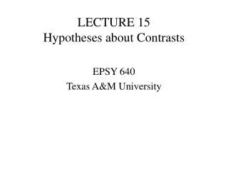
Polynomial Trend Contrasts 0 100 200 300 ml dose • C1 : -3 -1 1 3 linear • C2: -1 1 1 -1 quadratic • C3: -1 3 -3 1 cubic
C1 3 2 1 0 -1 -2 -3 3 2 1 0 -1 -2 -3 C3 3 2 1 0 -1 -2 -3 C2 0 100 200 300 0 100 200 300 0 100 200 300 Fig. 9.2: Graphs of planned orthogonal contrasts for four interval treatments
3 2 1 0 -1 -2 -3 0 100 200 300
ERROR RATES • EXPERIMENTWISE ERROR RATE- total error rate for all hypothesis tests • FAMILYWISE ERROR RATE- error rate within a set of hypothesis tests (eg. multiple comparisons for a given dependent variable)
POST HOC MULTIPLE COMPARISONS • Used after omnibus ANOVA significance • No preplanned hypotheses • Less power but good for exploration of a new result
POST HOC MULTIPLE COMPARISONS • Two types based on error rate: • contrast based: Duncan, Newman-Keuls • familywise based: Tukey, Scheffe, Bonferroni (Dunn), Dunn-Sjdak
TUKEY Procedure • Order groups by mean from high to low • Compute significant difference required for the number of groups • Compare each pair of groups for significance • Organize nonsignificant subsets of groups
Bonferroni Procedure • Allows both simple and complex contrasts • Set total familywise error rate you will accept • Divide the error rate by the number of contrasts to be evaluated: e/n (eg. .05/4) • Test each contrast as a t-test at that error rate (.0125 for the example above)
Design the experiment yes no Are there planned contrasts? yes Underlying continuum for groups? no Run ANOVA yes Are contrasts orthogonal? no STOP Significant? no Run Games- Howell procedure yes no equal variances? run Planned Orthogonal Contrasts Run Tukey’s procedure yes yes yes no Run trend contrasts run Dunn or Dunn-Sidak All contrasts simple? equal n’s? Run Sidak procedure no
PLANNED COMPARISONS • PLANNED • PLANNED ORTHOGONAL COMPARISONS • TREND COMPARISONS • DUNN NONORTHOGONAL COMPARISONS • POST HOC • ANOVA FIRST • COMPLEX, RUN DUNN • SIMPLE, RUN TUKEY (if equal sample sizes), or Sjdak if unequal, or Games-Howell if unequal variances across groups
ASSUMPTIONS • RANDOMIZATION OR • NORMALITY • EQUAL POPULATION VARIANCES FOR ALL GROUPS • INDEPENDENCE OF ERRORS
ASSUMPTIONS • ROBUSTNESS: • MODERATE SKEWNESS, KURTOSIS • EQUAL SAMPLE SIZES • VARIANCES BELOW 4:1 OR SO
ASSUMPTIONS • UNEQUAL SAMPLE SIZE: • Induces dependencies in data • not robust if variances unequal: • small sample-large variance • alpha level inflates greatly (Type I errors) • small sample-small variance • alpha level gets smaller (low power)